Machine Learning Fundamentals

Supervised learning

Supervised learning is a fundamental concept in machine learning, where an algorithm learns from labeled data to make predictions or decisions. In supervised learning, the algorithm is trained on a dataset consisting of input-output pairs, where the inputs (features) are associated with corresponding outputs (labels or target variables).

Here’s how supervised learning works:

Training Phase: During the training phase, the algorithm learns from the labeled dataset to create a model that can map inputs to outputs. The labeled dataset is divided into two parts: the training set and the validation set. The training set is used to train the model, while the validation set is used to evaluate the model’s performance and adjust hyperparameters.
Model Representation: The model learns a mapping function that approximates the relationship between the input features and the target variable. This mapping function can take various forms, depending on the specific algorithm used for supervised learning. For example, in linear regression, the mapping function is a linear equation, while in decision trees, it is a tree-like structure of decision rules.
Prediction Phase: Once the model is trained, it can be used to make predictions on new, unseen data. The model takes input features as input and generates predictions or decisions as output. The performance of the model is evaluated using metrics such as accuracy, precision, recall, or F1-score, depending on the nature of the problem (classification or regression) and the specific requirements.

Supervised learning can be further categorized into two main types:

Classification: In classification tasks, the target variable is categorical, meaning it belongs to a discrete set of classes or categories. The goal is to predict the class label of new instances based on their input features. Common algorithms for classification include logistic regression, decision trees, random forests, support vector machines (SVM), and neural networks.
Regression: In regression tasks, the target variable is continuous, meaning it can take any real-numbered value within a range. The goal is to predict a numerical value or quantity based on the input features. Linear regression, polynomial regression, decision trees, random forests, and neural networks are commonly used for regression tasks.

Supervised learning is widely used in various applications, including but not limited to:

Predictive analytics
Image classification
Speech recognition
Natural language processing
Recommender systems
Financial forecasting

Overall, supervised learning plays a crucial role in solving real-world problems by enabling machines to learn from labeled data and make intelligent decisions or predictions.

Unsupervised learning

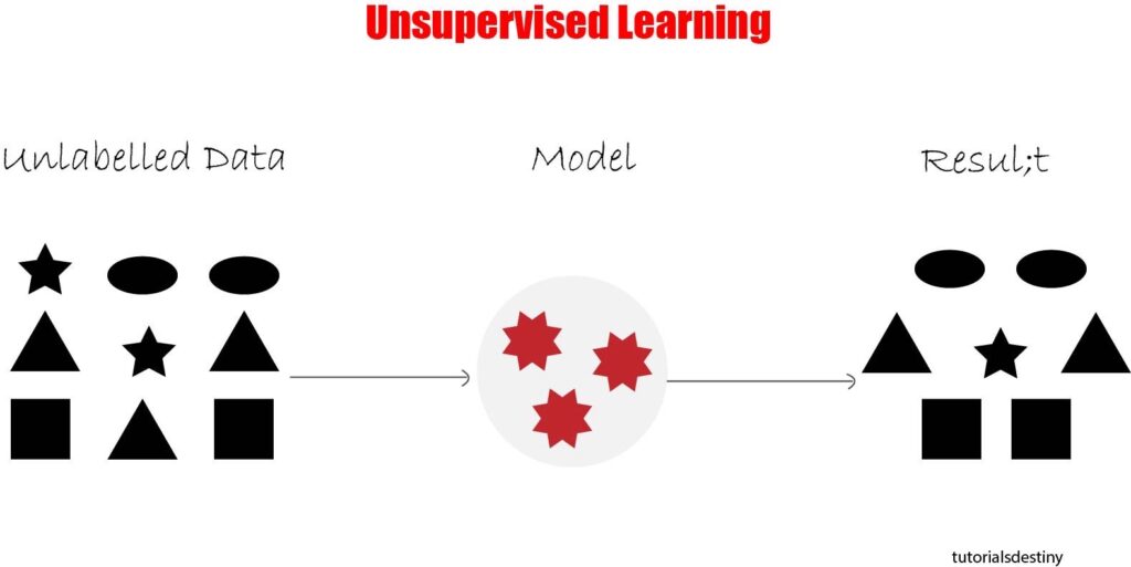
Unsupervised learning is a machine learning paradigm where the algorithm learns from unlabeled data to discover patterns, structures, or relationships within the data. Unlike supervised learning, unsupervised learning does not require labeled output data. Instead, the algorithm seeks to find inherent structures or hidden patterns within the input data.

Here’s how unsupervised learning works:

Training Phase: During the training phase, the algorithm is presented with a dataset consisting only of input features, without any corresponding output labels. This dataset is often referred to as an “unlabeled dataset.” The algorithm’s objective is to explore and identify meaningful patterns or structures within the data without explicit guidance or supervision.
Pattern Discovery: Unsupervised learning algorithms aim to uncover inherent structures or relationships within the data, such as clusters, associations, or anomalies. The algorithm may identify clusters of similar data points, discover associations between different features, or detect outliers or anomalies that deviate significantly from the norm.
Model Representation: The output of an unsupervised learning algorithm typically consists of learned representations or transformations of the input data. These representations capture the underlying structure or patterns within the data and can be used for various purposes, such as data visualization, dimensionality reduction, or feature engineering.
Evaluation: Unlike supervised learning, where performance can be evaluated using metrics such as accuracy or precision, evaluating the performance of unsupervised learning algorithms can be more challenging. Evaluation metrics depend on the specific task and objectives of the algorithm. For example, clustering algorithms may be evaluated based on clustering quality measures such as silhouette score or Davies-Bouldin index.

Unsupervised learning can be further categorized into several main types:

Clustering: Clustering algorithms group similar data points together into clusters based on their intrinsic similarities. Examples of clustering algorithms include k-means clustering, hierarchical clustering, and DBSCAN (Density-Based Spatial Clustering of Applications with Noise).
Dimensionality Reduction: Dimensionality reduction techniques aim to reduce the number of features or dimensions in the dataset while preserving as much relevant information as possible. Principal Component Analysis (PCA), t-Distributed Stochastic Neighbor Embedding (t-SNE), and Autoencoders are commonly used for dimensionality reduction.
Association Rule Learning: Association rule learning algorithms identify relationships or associations between different features or items in a dataset. These algorithms are commonly used in market basket analysis and recommendation systems to discover patterns in transactional data. Apriori and FP-Growth are examples of association rule learning algorithms.

Unsupervised learning has numerous applications across various domains, including but not limited to:

Anomaly detection
Customer segmentation
Image and text clustering
Data preprocessing and feature engineering
Recommender systems
Generative modeling and data synthesis

Overall, unsupervised learning plays a vital role in exploratory data analysis, pattern discovery, and knowledge discovery from unlabeled data, providing valuable insights and facilitating decision-making in diverse fields.

Reinforcement learning

Reinforcement learning (RL) is a type of machine learning where an agent learns to make decisions by interacting with an environment. The agent learns to achieve a specific goal or maximize cumulative rewards through a process of trial and error.

Here’s how reinforcement learning works:

Agent: The agent is the entity that learns to perform actions in an environment to achieve a goal. It makes decisions based on the information it receives from the environment and the rewards it receives for its actions.
Environment: The environment represents the external system with which the agent interacts. It provides feedback to the agent in the form of rewards and state transitions based on the agent’s actions.
Actions: At each time step, the agent selects an action from a set of possible actions available in the environment. The choice of action depends on the agent’s policy, which defines the mapping from states to actions.
States: The state represents the current situation or configuration of the environment. It captures relevant information that the agent uses to make decisions. The state can be discrete or continuous, depending on the nature of the problem.
Rewards: After taking an action in a particular state, the agent receives a reward from the environment. The reward indicates the immediate benefit or cost associated with the action. The goal of the agent is to maximize cumulative rewards over time.
Learning Process: The agent learns to improve its decision-making policy through experience. It explores different actions and observes the resulting rewards and state transitions. By associating actions with rewards and updating its policy accordingly, the agent learns to make better decisions over time.
Exploration vs. Exploitation: Reinforcement learning involves a trade-off between exploration and exploitation. Exploration involves trying out different actions to discover their effects and learn about the environment. Exploitation involves choosing actions that are known to yield high rewards based on the agent’s current knowledge. Balancing exploration and exploitation is essential for effective learning.

Reinforcement learning algorithms can be categorized into two main types:

Value-based methods: These methods learn a value function that estimates the expected cumulative reward of taking a particular action in a given state. Examples include Q-learning and Deep Q-Networks (DQN).
Policy-based methods: These methods learn a policy directly, without explicitly estimating value functions. They directly optimize the agent’s policy to maximize cumulative rewards. Examples include policy gradient methods like REINFORCE and actor-critic methods.

Reinforcement learning has applications in various domains, including robotics, game playing, finance, healthcare, and autonomous systems. It has been used to develop agents that can play games like chess, Go, and video games, control autonomous vehicles, and optimize business processes.

Overall, reinforcement learning provides a powerful framework for learning to make decisions in dynamic and uncertain environments, enabling agents to adapt and improve their behavior over time.

Evaluation and performance metrics

Evaluation and performance metrics are essential in assessing the effectiveness and quality of machine learning models and algorithms. These metrics provide insights into how well a model performs on a given task and help compare different models or approaches. Here are some common evaluation and performance metrics used in machine learning:

Accuracy: Accuracy measures the proportion of correctly classified instances out of the total number of instances. It is calculated as the ratio of true positives and true negatives to the total number of predictions. While accuracy is a commonly used metric, it may not be suitable for imbalanced datasets.
Precision: Precision measures the proportion of true positive predictions out of all positive predictions made by the model. It is calculated as the ratio of true positives to the sum of true positives and false positives. Precision is useful when the cost of false positives is high.
Recall (Sensitivity): Recall measures the proportion of true positive predictions out of all actual positive instances in the dataset. It is calculated as the ratio of true positives to the sum of true positives and false negatives. Recall is useful when the cost of false negatives is high.
F1 Score: The F1 score is the harmonic mean of precision and recall. It provides a balance between precision and recall and is useful when there is an imbalance between the two. The F1 score ranges from 0 to 1, with higher values indicating better performance.
ROC Curve (Receiver Operating Characteristic Curve): The ROC curve plots the true positive rate (recall) against the false positive rate for different threshold values. It provides a visual representation of the trade-off between sensitivity and specificity. The area under the ROC curve (AUC-ROC) is a common metric used to evaluate classification models, with higher values indicating better performance.
Confusion Matrix: A confusion matrix is a tabular representation of the predicted and actual classes in a classification problem. It provides insights into the performance of the model by showing the number of true positives, true negatives, false positives, and false negatives.
Mean Absolute Error (MAE) and Mean Squared Error (MSE): MAE and MSE are metrics used to evaluate regression models. MAE measures the average absolute difference between the predicted and actual values, while MSE measures the average squared difference. Lower values indicate better performance for both metrics.
R-squared (R^2) Score: The R-squared score measures the proportion of the variance in the dependent variable that is explained by the independent variables in a regression model. It ranges from 0 to 1, with higher values indicating better fit.

These are just a few examples of evaluation and performance metrics used in machine learning. The choice of metrics depends on the specific task, dataset, and objectives of the model. It’s essential to select appropriate metrics that align with the goals of the project and provide meaningful insights into the model’s performance.