
Q-Learning: Value-Based Reinforcement Learning
Q-Learning is a value-based method in reinforcement learning, which means it focuses on learning the value of actions taken in specific states. The “value” in this context refers to the expected long-term reward an agent can achieve by taking a certain action from a given state and then following an optimal policy in subsequent steps.
The Q-Function
In Q-Learning, the agent learns an estimate of the Q-function, which is defined as:
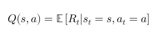
Here, ( Q(s, a) ) represents the expected reward the agent will receive by taking action ( a ) in state ( s ), and following the optimal policy thereafter. The goal of Q-Learning is to iteratively improve the estimate of this function so that the agent can act optimally.
How Q-Learning Works
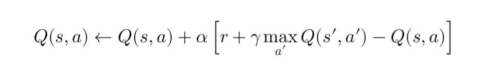
Q-Learning updates its Q-values using the Bellman equation, which defines the relationship between the value of the current state-action pair and the future state:
Where:
- ( s ) is the current state,
- ( a ) is the current action,
- ( r ) is the reward,
- ( s’ ) is the next state,
- ( \gamma ) is the discount factor (indicating how much future rewards are valued),
- ( \alpha ) is the learning rate.
At each step, the agent updates the Q-value for the current state-action pair based on the immediate reward ( r ) and the maximum Q-value for the next state ( s’ ). Over time, this process allows the Q-function to converge to the true value of actions, helping the agent make more informed decisions.
Exploration vs. Exploitation
A key concept in Q-Learning is the balance between exploration and exploitation. While exploitation involves selecting actions based on the learned Q-values (to maximize reward), exploration refers to trying new actions to discover potentially better strategies. This is often managed using an epsilon-greedy strategy, where the agent explores with probability ( \epsilon ) and exploits with probability ( 1 – \epsilon ).
Strengths and Limitations of Q-Learning
Strengths:
- Model-free: Q-Learning does not require a model of the environment, making it adaptable to complex problems.
- Off-policy: It can learn from previous experiences and explore off-policy, meaning it can learn the optimal policy even if the agent does not follow the optimal policy during learning.
Limitations:
- Scalability: Q-Learning struggles with high-dimensional state or action spaces. In complex environments, maintaining and updating a Q-table for every state-action pair becomes computationally prohibitive.
- Continuous Actions: Q-Learning works well for discrete action spaces but is difficult to extend to environments with continuous actions.
Policy Gradients: Policy-Based Reinforcement Learning
Unlike Q-Learning, which learns value estimates, Policy Gradients directly optimize the policy that governs the agent’s actions. Instead of learning a Q-function, policy gradients learn a parameterized policy that maps states to actions.
The Policy Function
The policy, denoted ( \pi(a|s; \theta) ), is a probability distribution over actions, given a state ( s ) and parameters ( \theta ). The goal of policy gradients is to directly maximize the expected cumulative reward by adjusting the policy’s parameters through gradient ascent.
The objective is to maximize the expected return ( J(\theta) ), which is defined as:
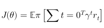
Where ( \gamma ) is the discount factor, and ( r_t ) is the reward at time step ( t ).
How Policy Gradients Work
Policy gradient methods use the REINFORCE algorithm (Williams, 1992), a form of stochastic gradient ascent. The update rule for the policy parameters is given by:
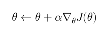
The gradient ( \nabla_{\theta} J(\theta) ) is computed using:
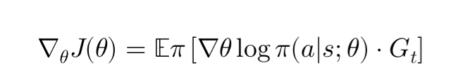
Where ( G_t ) is the return from time step ( t ). This equation indicates that the gradient of the policy is scaled by the return of the episode, so actions that lead to higher rewards will have their probabilities increased.
Strengths and Limitations of Policy Gradients
Strengths:
- Continuous Actions: Policy gradients work well in environments with continuous action spaces, unlike Q-Learning.
- Stochastic Policies: Policy gradients allow for stochastic policies, which can be advantageous in environments with uncertainty or where exploration is important.
- Direct Optimization: Since policy gradients directly optimize the policy, they can sometimes converge more smoothly in complex environments than value-based methods.
Limitations:
- High Variance: Policy gradients often suffer from high variance in the gradient estimates, making learning unstable and slow.
- Sample Inefficiency: Policy gradient methods typically require a large number of samples to learn effectively, especially in environments with sparse rewards.
- On-policy: Policy gradients are typically on-policy, meaning the agent must interact with the environment to improve the current policy, which can be less efficient compared to off-policy methods like Q-Learning.
Comparing Q-Learning and Policy Gradients
| Feature | Q-Learning | Policy Gradients |
|---|---|---|
| Approach | Value-based (estimates Q-values) | Policy-based (optimizes policy directly) |
| Action Space | Best for discrete action spaces | Handles both discrete and continuous actions |
| Policy Type | Deterministic (selects max Q-value action) | Can be stochastic or deterministic |
| Learning Type | Off-policy | On-policy |
| Exploration | Epsilon-greedy exploration | Inherent to stochastic policies |
| Sample Efficiency | More sample efficient | Requires more data for training |
| Variance in Learning | Lower variance in updates | High variance in gradient estimates |
When to Use Q-Learning vs. Policy Gradients
- Q-Learning is preferable for problems with discrete action spaces and where computational resources are limited. Its off-policy nature allows for more flexible learning from past experiences and exploration.
- Policy Gradients are suitable for problems with continuous action spaces or where stochastic behavior is necessary. They directly optimize the policy, making them a better fit for complex, high-dimensional problems, despite their sample inefficiency and high variance.
Conclusion
Both Q-Learning and Policy Gradients are powerful tools in the reinforcement learning toolbox, each suited to different types of problems. Q-Learning excels in environments with discrete actions and offers efficient learning through value iteration. Policy gradients, on the other hand, shine in continuous action spaces and can handle more complex, stochastic decision-making scenarios.
By understanding the strengths and limitations of each approach, practitioners can select the most appropriate algorithm for their specific reinforcement learning challenges.