Introduction
In this module, we delve into the techniques and metrics used to evaluate machine learning models. Understanding metrics and validation ensures that your model is both accurate and generalizable, minimizing errors when deployed in real-world scenarios.
Why Are Metrics and Validation Crucial?
- Accuracy Alone Is Not Enough: A high accuracy score can be misleading, especially in imbalanced datasets. You need comprehensive metrics to capture model performance accurately.
- Prevents Overfitting/Underfitting: Proper validation techniques highlight issues with generalizability.
- Enables Model Comparison: Metrics allow you to benchmark different models effectively.
1. Classification Metrics
Classification metrics measure the performance of models that predict discrete outcomes.
Examples:
Scenario: Spam Email Classification
- Dataset: Emails labeled as “Spam” or “Not Spam.”
- Positive Class: “Spam”
Metrics:
- Accuracy: Proportion of correct predictions (both spam and not spam).
\[Formula: ( \text{Accuracy} = \frac{\text{True Positives} + \text{True Negatives}}{\text{Total Predictions}} ) \] - Example: 90 correct predictions out of 100 emails → Accuracy = 90%.
- Limitation: Accuracy is misleading in imbalanced datasets.
- Precision: Focuses on the correctness of positive predictions.
\[Formula: ( \text{Precision} = \frac{\text{True Positives}}{\text{True Positives} + \text{False Positives}} )\] - Example: Out of 40 emails predicted as spam, 36 were correct →
\(Precision = ( \frac{36}{40} = 90\% ).\)
- Example: Out of 40 emails predicted as spam, 36 were correct →
- Recall (Sensitivity): Measures how many actual positives the model identified.
\[Formula: ( \text{Recall} = \frac{\text{True Positives}}{\text{True Positives} + \text{False Negatives}} )\] - Example: 50 spam emails exist, and 36 were detected →
\(Recall = ( \frac{36}{50} = 72\% ).\)
- Example: 50 spam emails exist, and 36 were detected →
- F1-Score: The harmonic mean of precision and recall, balancing both.
\[Formula: ( \text{F1-Score} = 2 \times \frac{\text{Precision} \times \text{Recall}}{\text{Precision} + \text{Recall}} )\] - AUC-ROC Curve: Evaluates model performance across different classification thresholds.
- Example: Comparing two spam filters, the one with an AUC-ROC closer to 1 is more effective at separating spam from non-spam.
2. Regression Metrics
Regression metrics measure the performance of models predicting continuous outcomes.
Choosing Metrics Based on Business Goals:
- MAE: Suitable when all errors are equally penalized, such as predicting delivery times.
- RMSE: Use when larger errors are more critical, e.g., predicting costs or financial losses.
- R² Score: Helps stakeholders understand the explanatory power of the model.
Example: Predicting House Prices
- Dataset: Features like size, location, and number of bedrooms predict house prices.
Metrics:
- Mean Absolute Error (MAE): Measures the average magnitude of errors in predictions.
\[Formula: ( \text{MAE} = \frac{1}{n} \sum_{i=1}^n |y_i – \hat{y}_i| )\] - Example: Actual prices = [100k, 200k, 300k], Predictions = [110k, 190k, 310k].
- Errors: [10k, 10k, 10k].
\(MAE = ( \frac{10k + 10k + 10k}{3} = 10k ).\)
- Example: Actual prices = [100k, 200k, 300k], Predictions = [110k, 190k, 310k].
- Root Mean Squared Error (RMSE): Penalizes larger errors more than
MAE.
\[Formula: ( \text{RMSE} = \sqrt{\frac{1}{n} \sum_{i=1}^n (y_i – \hat{y}_i)^2} )\] - R² Score: Explains how much variance in the target variable is captured by the model.
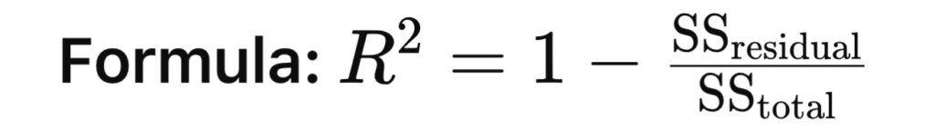
- Example: An
\( R^2 \) of 0.9 means the model explains 90% of the variation in house prices.
Advanced Example: Energy Consumption Prediction
- Predicting daily energy consumption for a household.
- Actual: [50, 60, 65, 70], Predicted: [52, 58, 67, 68]
\(MAE = 2.5, RMSE = 3.0, R2=0.92R2=0.92.\) - Insight: MAE and RMSE indicate small errors, and R2R2 confirms the model explains 92% of the variability.
Practical Tip: Visualize actual vs. predicted values to identify systematic errors:
import matplotlib.pyplot as plt<br><br>plt.scatter(y_test, y_pred)<br>plt.xlabel("Actual Values")<br>plt.ylabel("Predicted Values")<br>plt.title("Actual vs Predicted")<br>plt.show()<br><br><br>3. Clustering Metrics
Clustering metrics evaluate models that group data points into clusters.
Example: Customer Segmentation for Marketing
- Dataset: Customer data with attributes like age, income, and purchase history.
Metrics:
- Silhouette Score: Measures how similar a point is to its own cluster compared to others.
- Range: -1 (poor clustering) to 1 (excellent clustering).
- Example: A silhouette score of 0.8 indicates well-separated clusters.
- Davies-Bouldin Index:
- Evaluates cluster compactness and separation.
- Lower values indicate better clustering.
- Adjusted Rand Index (ARI):
- Compares clustering results with true labels.
- Example: Segmenting customers into age-based clusters, ARI shows how well these match actual age groups.
4. Validation Techniques
Validation ensures your model generalizes well to unseen data.
Techniques:
- Train-Test Split:
- Example: For a dataset with 1,000 entries, allocate 80% for training and 20% for testing.
- K-Fold Cross-Validation:
- Splits the dataset into ( k ) subsets, using ( k-1 ) for training and 1 for testing, rotating the subsets.
- Example: For ( k = 5 ), 5 iterations are performed, each with a different test subset.
- Stratified K-Fold:
- Ensures class balance is maintained during splits.
- Example: In a binary classification problem with 70% positives and 30% negatives, each fold maintains this ratio.
- Bootstrapping:
- Random sampling with replacement to create multiple datasets for evaluation.
- Example: In medical data analysis, bootstrapping provides robust confidence intervals for model predictions.
Advanced Example: Stratified K-Fold in Imbalanced Data
- Dataset: 1,000 samples, 900 negatives, 100 positives.
- In regular K-Fold, a fold may have 95% negatives, leading to biased evaluation.
- Stratified K-Fold ensures each fold has 90% negatives and 10% positives, preserving the dataset’s class balance.
Practical Tip: Implement Stratified K-Fold using Scikit-learn:
from sklearn.model_selection import StratifiedKFold

skf = StratifiedKFold(n_splits=5)
for train_index, test_index in skf.split(X, y):
    print("Train:", train_index, "Test:", test_index)
Common Pitfalls to Avoid
- Ignoring Imbalanced Data: Always analyze class distributions before selecting metrics.
- Over-relying on a Single Metric: Use a combination of metrics (e.g., precision, recall, and F1-score) for a comprehensive evaluation.
- Skipping Validation: Train-test split alone isn’t enough; use cross-validation for robust evaluations.
- Not Considering Business Context: Always align metrics with the problem’s real-world implications.
Final Takeaway
Metrics and validation form the backbone of reliable machine learning. Whether it’s classification, regression, or clustering, always choose metrics and techniques that align with your dataset and business objectives. By using these insights, your models will perform effectively and generalised well to unseen data.