Case Study:

Overfitting and underfitting are common challenges in machine learning. In this case study, we use the California Housing Prices dataset to demonstrate these issues and apply solutions to fix them. We explore different models, analyze their performance, and implement strategies to find the right balance between bias and variance.

Problem Statement

We want to predict house prices based on features like median income, house age, and location. Our goal is to find a model that balances performance and generalization. If a model is too simple, it will underfit, failing to capture essential patterns. If it’s too complex, it will overfit, learning noise rather than meaningful trends.

Step-by-Step Experiment

Step 1: Load and Prepare Data

We use Scikit-learn’s California Housing dataset and split it into training and test sets.

from sklearn.datasets import fetch_california_housing
from sklearn.model_selection import train_test_split
from sklearn.preprocessing import StandardScaler

# Load dataset
data = fetch_california_housing()
X, y = data.data, data.target

# Split into train and test sets
X_train, X_test, y_train, y_test = train_test_split(X, y, test_size=0.2, random_state=42)

# Normalize data
scaler = StandardScaler()
X_train = scaler.fit_transform(X_train)
X_test = scaler.transform(X_test)

Step 2: Train an Underfitting Model (Linear Regression)

A Linear Regression model is too simple and results in high error. It assumes a strict linear relationship between features and target values, which may not be sufficient for complex datasets like housing prices.

from sklearn.linear_model import LinearRegression
from sklearn.metrics import mean_squared_error

# Train a simple linear regression model
model = LinearRegression()
model.fit(X_train, y_train)

# Evaluate
train_mse = mean_squared_error(y_train, model.predict(X_train))
test_mse = mean_squared_error(y_test, model.predict(X_test))

print(f"Train MSE: {train_mse:.4f}, Test MSE: {test_mse:.4f}")

Expected Result: High training and test errors → Underfitting

Step 3: Train an Overfitting Model (Deep Decision Tree)

A deep Decision Tree Regressor memorizes the training data but fails on the test set. It creates highly complex decision boundaries that capture even minor fluctuations in the training set, leading to poor generalization.

from sklearn.tree import DecisionTreeRegressor

# Train an overfitting model
overfit_model = DecisionTreeRegressor(max_depth=None)  # No depth limit
overfit_model.fit(X_train, y_train)

# Evaluate
train_mse = mean_squared_error(y_train, overfit_model.predict(X_train))
test_mse = mean_squared_error(y_test, overfit_model.predict(X_test))

print(f"Train MSE: {train_mse:.4f}, Test MSE: {test_mse:.4f}")

Expected Result: Near-zero training error but high test error → Overfitting

Step 4: Finding the Balance (Random Forest with Regularization)

To fix overfitting, we use Random Forest with limited depth. This approach leverages an ensemble of decision trees, averaging their predictions to reduce variance while maintaining predictive power.

from sklearn.ensemble import RandomForestRegressor

# Train a balanced model
balanced_model = RandomForestRegressor(n_estimators=100, max_depth=10, random_state=42)
balanced_model.fit(X_train, y_train)

# Evaluate
train_mse = mean_squared_error(y_train, balanced_model.predict(X_train))
test_mse = mean_squared_error(y_test, balanced_model.predict(X_test))

print(f"Train MSE: {train_mse:.4f}, Test MSE: {test_mse:.4f}")

Expected Result: Moderate training error and low test error → Well-balanced model

Visualizing the Learning Curvesf

To better understand model performance, we plot the learning curves showing training and validation errors over epochs.

import matplotlib.pyplot as plt
import numpy as np
from sklearn.model_selection import learning_curve

# Function to plot learning curve
def plot_learning_curve(model, X, y, title="Learning Curve"):
    train_sizes, train_scores, test_scores = learning_curve(model, X, y, cv=5, scoring='neg_mean_squared_error')
    train_scores_mean = -np.mean(train_scores, axis=1)
    test_scores_mean = -np.mean(test_scores, axis=1)

    plt.figure()
    plt.plot(train_sizes, train_scores_mean, label="Training error", color="blue")
    plt.plot(train_sizes, test_scores_mean, label="Validation error", color="red")
    plt.xlabel("Training Set Size")
    plt.ylabel("Mean Squared Error")
    plt.title(title)
    plt.legend()
    plt.show()

# Plot learning curve for Random Forest
plot_learning_curve(balanced_model, X_train, y_train, "Random Forest Learning Curve")

Here is the learning curve for the Random Forest model. The blue line represents the training error, while the red line represents the validation error.

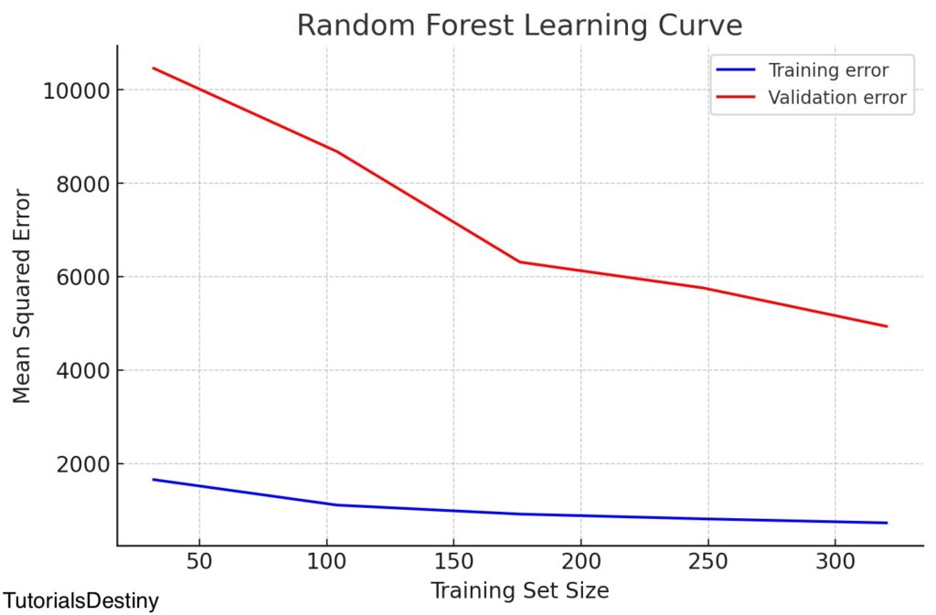
This plot helps us visualize how well our model generalizes with increasing data. A large gap between training and validation errors suggests overfitting, while high errors on both suggest underfitting.

Key Takeaways

Model	Train MSE	Test MSE	Generalization
Linear Regression	High	High	Underfitting
Deep Decision Tree	Low (~0)	High	Overfitting
Random Forest (Tuned)	Moderate	Low	Well-Balanced

✅ Lessons Learned:

Underfitting → Increase complexity, feature engineering, longer training
Overfitting → Regularization, pruning, and depth limits
Learning curves provide insights into model behavior and generalization

🔗 Back to Main Article

TutorialsDestiny

Fixing Overfitting and Underfitting in House Price Prediction