Category: Quantum computer

  • Quantum Tunneling: When Particles Break the Rules of Classical Reality

    Quantum Tunneling: When Particles Break the Rules of Classical Reality

    Introduction

    In our everyday experience, physical objects follow strict and predictable rules. A ball thrown at a wall bounces back, and a car cannot cross a barrier without breaking through it. These observations form the foundation of classical physics, which governs the macroscopic world. Classical mechanics assumes that objects have definite positions, energies, and trajectories, and that motion is fully determined by forces and energy conservation.

    However, when we move from the visible world to the microscopic realm of atoms, electrons, and subatomic particles, these familiar rules begin to fail. Nature behaves in ways that are often counter-intuitive and probabilistic rather than deterministic. One of the most fascinating phenomena arising from this quantum domain is quantum tunneling—a process in which particles pass through energy barriers that they seemingly should not be able to cross.

    Quantum tunneling is not merely a theoretical curiosity. It is a fundamental mechanism behind nuclear fusion in stars, radioactive decay, modern electronic devices, and advanced scientific instruments. This phenomenon challenges classical intuition and reveals the true nature of reality at the smallest scales.

    Understanding Quantum Tunneling

    At its core, quantum tunneling refers to the phenomenon where a particle has a non-zero probability of passing through a potential energy barrier, even when its total energy is less than the height of that barrier.

    In classical physics:i

    • A particle approaching a barrier with insufficient energy must be reflected.
    • The probability of crossing the barrier is strictly zero.

    Quantum mechanics, however, introduces probability as a fundamental aspect of nature. According to this framework, particles are described by wavefunctions, mathematical entities that provide information about the likelihood of finding a particle at a particular position.

    When a particle encounters a barrier:

    • Its wavefunction does not abruptly end at the boundary.
    • Instead, it penetrates into the barrier and decays exponentially.
    • If the barrier is thin enough, the wavefunction may extend beyond it, allowing the particle to appear on the other side.

    This process—where a particle effectively “passes through” a barrier without climbing over it—is known as quantum tunneling.

    Wave–Particle Duality: The Foundation of Tunneling

    Quantum tunneling is a direct consequence of wave–particle duality, one of the central principles of quantum mechanics. According to this principle:

    • Every particle exhibits both particle-like and wave-like behavior.
    • Electrons, protons, and even atoms can behave as waves under certain conditions.

    Unlike classical particles, waves do not have sharply defined positions. They spread out over space, allowing parts of the wave to exist in regions that would be forbidden for a classical particle. When a quantum particle approaches a barrier, its wavefunction spreads into the barrier region, making tunneling possible.

    This dual nature challenges our classical intuition but provides a more accurate description of the microscopic universe.

    A Simple Analogy to Visualize Tunneling

    To visualize quantum tunneling, imagine rolling a ball toward a hill.

    • In classical physics, the ball must have enough energy to climb over the hill.
    • If it lacks sufficient energy, it rolls back.

    In quantum physics, the “ball” behaves like a wave:

    • The wave spreads out as it approaches the hill.
    • A portion of the wave may appear on the other side.
    • When measured, the particle may be detected beyond the barrier.

    The particle does not physically climb the hill—it tunnels through it.

    Classical vs Quantum Mechanics

    Classical View

    According to classical mechanics, the kinetic energy of a particle is:

    \[K = \frac{1}{2}mv^2\]

    Since:

    • Mass \(m\) is always positive
    • Velocity squared \(v^2\) is always positive

    Kinetic energy can never be negative. If a particle encounters a potential barrier of height \(V_0\) and its total energy \(E < V_0\), then its kinetic energy inside the barrier would be negative—an impossible situation in classical physics. Hence, total reflection is predicted.

    Quantum Mechanical View

    Quantum mechanics allows total reflection only when the barrier height is infinite. For a finite potential barrier, even if \(E < V_0\), there is a finite probability that the particle will appear on the other side.

    This crucial difference gives rise to quantum tunneling.

    Mathematical Perspective (Conceptual)

    Quantum behavior is governed by the time-independent Schrödinger equation (TISE):

    \[\frac{d^2 \psi}{dx^2} + \frac{2m}{\hbar^2}(E – V)\psi = 0\]

    Here:

    • \(\psi(x)\) is the wavefunction
    • \(|\psi(x)|^2 \)represents probability density
    • \(E\) is total energy
    • \(V(x)\) is potential energy

    The Schrödinger equation predicts that the wavefunction decays exponentially inside a barrier but does not become zero, allowing tunneling to occur.

    Quantum Mechanical Tunneling: Potential Barrier Model

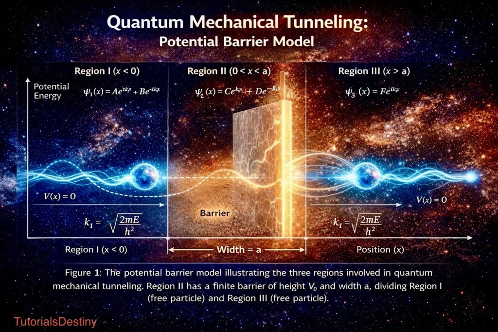
    To understand tunneling rigorously, consider a one-dimensional finite potential barrier divided into three regions.

    Potential Definition

    \[V(x) = \begin{cases} 0, & x < 0 \quad \text{(Region I)} \\ V_0, & 0 \le x \le a \quad \text{(Region II)} \\ 0, & x > a \quad \text{(Region III)} \end{cases}\]

    where:

    • \(V_0\) is the barrier height
    • \(a\) is the barrier width
    • \(E < V_0\)

    Region I: \( x < 0\) (Incident and Reflected Waves)

    The Schrödinger equation becomes:

    \[\frac{d^2 \psi}{dx^2} + k_1^2 \psi = 0\]

    where:

    \[k_1 = \sqrt{\frac{2mE}{\hbar^2}}\]

    The solution is:

    \[\psi_1(x) = A e^{ik_1 x} + B e^{-ik_1 x}\]

    • First term: incident wave
    • Second term: reflected wave

    Region II: \(0 < x < a\) (Inside the Barrier)

    Here, \(E < V_0\), so the equation becomes:

    \[\frac{d^2 \psi}{dx^2} – k_2^2 \psi = 0\]

    with:

    \[k_2 = \sqrt{\frac{2m(V_0 – E)}{\hbar^2}}\]

    The solution is:

    \[\psi_2(x) = C e^{k_2 x} + D e^{-k_2 x}\]

    This region features exponentially decaying wavefunctions, representing barrier penetration.

    Region III: \( x > a\) (Transmitted Wave)

    The equation again becomes:

    \[\frac{d^2 \psi}{dx^2} + k_1^2 \psi = 0\]

    The solution is:

    \[\psi_3(x) = F e^{ik_1 x}\]

    Only a transmitted wave exists here; no wave travels backward.

    Transmission and Reflection Coefficients

    Applying boundary conditions at \(x = 0\) and \(x = a\), the transmission coefficient is obtained as:

    \[T = \frac{1}{1 + \frac{V_0^2}{4E(V_0 – E)} \sinh^2(k_2 a)}\]

    This expression shows that:

    • \(T \neq 0\) even when \(E < V_0\)
    • Tunneling probability decreases with increasing barrier width and height
    • Lighter particles tunnel more easily

    Quantum Tunneling in Nature

    1. Nuclear Fusion in the Sun

    Quantum tunneling is essential for the energy production in stars. Inside the Sun:

    • Protons repel each other due to electrostatic forces.
    • Classically, their thermal energy is insufficient to overcome this repulsion.
    • Quantum tunneling allows protons to approach closely enough for the strong nuclear force to bind them.

    This process enables nuclear fusion, releasing vast amounts of energy that power the Sun and sustain life on Earth. Without quantum tunneling, stars would not shine.

    2. Radioactive Alpha Decay

    In radioactive nuclei:

    • Alpha particles are trapped inside the nucleus by a strong potential barrier.
    • Classical physics predicts they should remain confined indefinitely.
    • Quantum tunneling allows them to escape.

    This escape results in alpha decay, a fundamental form of radioactivity. The rate of decay depends on the tunneling probability, which explains why different radioactive elements have different half-lives.

    Technological Applications of Quantum Tunneling

    1. Scanning Tunneling Microscope (STM)

    The scanning tunneling microscope is one of the most direct technological applications of quantum tunneling. It operates by:

    • Bringing a sharp metallic tip extremely close to a surface.
    • Applying a small voltage between the tip and the surface.
    • Measuring the tunneling current produced by electrons.

    This current is highly sensitive to distance, allowing scientists to image individual atoms. The STM revolutionized surface science and nanotechnology.

    2. Semiconductor Devices

    Quantum tunneling plays a crucial role in modern electronics, especially as devices shrink to nanometer scales.

    Applications include:

    • Tunnel diodes
    • Flash memory
    • Transistors in integrated circuits

    As components become smaller, tunneling effects become unavoidable. Engineers must carefully design devices to either utilize or suppress tunneling, depending on the application.

    3. Quantum Computing

    In quantum computing:

    • Tunneling enables particles to transition between quantum states.
    • It plays a role in quantum annealing and optimization algorithms.

    Quantum tunneling allows quantum computers to explore solution spaces more efficiently than classical computers for certain problems.

    Importance of Quantum Tunneling

    Quantum tunneling is not merely a theoretical concept. Its importance lies in its ability to:

    • Explain phenomena that classical physics cannot
    • Enable advanced experimental techniques
    • Drive technological innovation
    • Deepen our understanding of the quantum nature of reality

    It demonstrates that probability, rather than certainty, governs the microscopic world.

    Limitations and Common Misconceptions

    Despite its extraordinary nature, quantum tunneling has clear limitations:

    • It does not allow macroscopic objects to pass through walls.
    • The tunneling probability for large objects is effectively zero.
    • It does not violate conservation of energy or physical laws.

    Quantum tunneling is significant only at atomic and subatomic scales.

    Philosophical Implications

    Quantum tunneling raises profound philosophical questions about determinism and reality. It suggests that:

    • Nature is fundamentally probabilistic.
    • Events are governed by likelihood rather than certainty.
    • Observation plays a critical role in determining outcomes.

    These ideas challenge classical notions of causality and determinism.

    Conclusion

    Quantum tunneling stands as one of the most striking and beautiful phenomena in physics. It reveals a universe where particles behave as waves, barriers are not absolute, and the impossible becomes possible—at least with some probability. From powering the stars to enabling cutting-edge technology, quantum tunneling silently shapes both the cosmos and our everyday lives.

    By challenging our intuition and expanding our understanding of nature, quantum tunneling reminds us that reality at its deepest level is far richer and stranger than it appears.

    In the quantum world, even the gimpossible has a chance.

  • Understanding the Random Forest Algorithm: A Powerful Machine Learning Technique

    Random Forest is one of the most powerful and widely used machine learning algorithms. Known for its accuracy, versatility, and robustness, it is an ensemble learning method that builds multiple decision trees and combines their outputs to improve performance. In this article, we’ll break down how Random Forest works, its advantages, disadvantages, a comparison with decision trees, and when to use it in real-world applications.

    What is the Random Forest Algorithm?

    Random Forest is an ensemble learning method that constructs multiple decision trees and aggregates their results to enhance accuracy and minimize overfitting. It can be used for both classification and regression tasks.

    How Does It Work?

    1. Bootstrap Sampling (Bagging):
      • The algorithm randomly selects subsets of the training data (with replacement).
      • Each subset is used to train an individual decision tree.
    2. Feature Randomness:
      • Instead of considering all features, Random Forest selects a random subset of features at each split.
      • This ensures diverse trees, improving generalization.
    3. Majority Voting (Classification) / Averaging (Regression):
      • For classification, the final prediction is based on majority voting across all trees.
      • For regression, it takes the average of predictions from all trees.

    Advantages of Random Forest

    Reduces Overfitting: Unlike individual decision trees, Random Forest generalizes well to unseen data.
    Handles Missing Data: It can handle missing values and maintain good performance.
    Works Well with Large Datasets: Scales efficiently with high-dimensional data.
    Can Handle Both Categorical and Numerical Data: Flexible for various ML tasks.
    Feature Importance: Provides insights into which features are most significant.


    Disadvantages of Random Forest

    Computationally Expensive: Training a large number of trees requires more time and resources.
    Less Interpretability: Unlike a single decision tree, the results of Random Forest are not easily interpretable.
    Slower Predictions: Since multiple trees contribute to the final prediction, inference time is higher compared to a single decision tree.
    Memory Intensive: Requires more storage and RAM due to multiple trees being stored in memory.


    Comparison: Random Forest vs. Decision Tree

    FeatureDecision TreeRandom Forest
    ComplexitySimple and easy to interpretMore complex and less interpretable
    OverfittingProne to overfittingReduces overfitting significantly
    Computation SpeedFaster training and inferenceSlower due to multiple trees
    AccuracyCan be less accurate on complex dataHigher accuracy due to ensemble
    InterpretabilityEasy to understandHarder to interpret due to multiple trees
    ScalabilitySuitable for small datasetsWorks well with large datasets
    Memory UsageLowHigh due to multiple trees

    When Should You Use Random Forest?

    Random Forest is a powerful algorithm applicable to various industries and problem domains, including:

    🔹 Predicting customer churn – Helps businesses retain customers by identifying risk factors.
    🔹 Fraud detection in finance – Recognizes fraudulent transactions with high accuracy.
    🔹 Medical diagnosis & disease prediction – Assists in detecting conditions based on medical data.
    🔹 Stock market prediction – Analyzes past data trends to forecast stock movements.
    🔹 Image classification & object detection – Enhances accuracy in computer vision tasks.


    Implementing Random Forest in Python

    Using scikit-learn, you can quickly build and train a Random Forest model:

    from sklearn.ensemble import RandomForestClassifier
    from sklearn.datasets import load_iris
    from sklearn.model_selection import train_test_split
    from sklearn.metrics import accuracy_score
    
    # Load dataset
    data = load_iris()
    X_train, X_test, y_train, y_test = train_test_split(data.data, data.target, test_size=0.2, random_state=42)
    
    # Train the model
    model = RandomForestClassifier(n_estimators=100, random_state=42)
    model.fit(X_train, y_train)
    
    # Make predictions
    y_pred = model.predict(X_test)
    
    # Evaluate accuracy
    print("Accuracy:", accuracy_score(y_test, y_pred))

    Final Thoughts

    Random Forest is an excellent choice for many real-world problems due to its high accuracy, resilience to overfitting, and ability to handle diverse data types. However, it can be computationally expensive and less interpretable compared to a single decision tree. Whether you’re working on classification or regression, this algorithm provides reliable results and interpretability.

    🚀 Want to dive deeper into AI and machine learning?
    Enroll in our Comprehensive AI Course and master industry-leading techniques today!

    📌 Stay updated with the latest in AI and data science by following our blog!

    MachineLearning #RandomForest #AI #DataScience

  • Hands-on Guide to Simulating Quantum Systems and Integrating AI

    Introduction

    Quantum systems exhibit properties like superposition and entanglement, which can be simulated using quantum computing frameworks. AI can enhance quantum simulations by optimizing circuits, predicting quantum states, and improving error correction.

    Tools Required

    • Quantum Computing Frameworks:
      • IBM Qiskit (Python-based)
      • Google Cirq
      • Microsoft Q#
    • AI Libraries:
      • TensorFlow / PyTorch (for deep learning)
      • Scikit-learn (for classical ML models)
      • Quantum Machine Learning (QML) libraries like PennyLane

    Setting Up the Environment

    pip install qiskit pennylane tensorflow numpy matplotlib

    Simulating a Quantum System

    Example: Simulating a 2-Qubit System in Qiskit

    from qiskit import QuantumCircuit, Aer, transpile, assemble, execute
    import numpy as np
    import matplotlib.pyplot as plt
    
    # Create a quantum circuit with 2 qubits
    qc = QuantumCircuit(2)
    
    # Apply a Hadamard gate to create superposition
    qc.h(0)
    
    # Apply a CNOT gate for entanglement
    qc.cx(0, 1)
    
    # Visualize the circuit
    qc.draw('mpl')
    plt.show()
    
    # Simulate the quantum circuit
    simulator = Aer.get_backend('statevector_simulator')
    compiled_circuit = transpile(qc, simulator)
    job = execute(compiled_circuit, simulator)
    result = job.result()
    
    # Get state vector
    statevector = result.get_statevector()
    print("Quantum State Vector:", statevector)

    Integrating AI with Quantum Simulation

    Using a Neural Network to Predict Quantum States

    import tensorflow as tf
    from tensorflow.keras.models import Sequential
    from tensorflow.keras.layers import Dense
    
    # Generate training data: quantum states and their measurements
    X_train = np.random.rand(1000, 2)  # Random quantum states
    Y_train = np.sin(np.pi * X_train)  # Simulated measurements
    
    # Define a simple neural network
    model = Sequential([
        Dense(10, activation='relu', input_shape=(2,)),
        Dense(10, activation='relu'),
        Dense(2, activation='linear')
    ])
    
    # Compile and train the model
    model.compile(optimizer='adam', loss='mse')
    model.fit(X_train, Y_train, epochs=50, batch_size=32)
    
    # Predict quantum measurements for new states
    X_test = np.random.rand(10, 2)
    predictions = model.predict(X_test)
    print("Predicted Quantum Measurements:", predictions)

    Expanding to Real-World Applications

    • Quantum Machine Learning (QML): Train AI models on quantum-generated datasets.
    • Hybrid Quantum-Classical AI: Combine classical deep learning with quantum feature selection.
    • Optimization Problems: Use quantum annealing for AI-based optimization.

    Conclusion

    Simulating quantum systems with Qiskit and integrating AI enables innovative solutions in quantum computing. Further exploration can include Variational Quantum Circuits (VQCs) and hybrid AI-quantum models.

  • Quantum Cryptography: The Ultimate Frontier of Secure Communication

    Quantum Cryptography: The Ultimate Frontier of Secure Communication

    Introduction

    As digital security threats evolve, the world is moving toward quantum cryptography, a revolutionary approach to cybersecurity that leverages the principles of quantum mechanics. Unlike traditional encryption methods that rely on mathematical complexity, quantum cryptography provides unbreakable security based on the laws of physics.

    With the emergence of quantum computers, which can potentially break classical encryption systems like RSA and ECC, governments, businesses, and researchers are racing to develop and deploy quantum-secure encryption.

    In this article, we will dive deep into quantum cryptography, exploring its principles, technologies, advantages, challenges, and real-world applications.

    Understanding Quantum Cryptography

    Quantum cryptography is a branch of cryptographic science that utilities quantum mechanics to encrypt and transmit data securely. The key difference between quantum cryptography and classical cryptography lies in how information is secured:

    Classical Cryptography: Relies on computational complexity (e.g., factorisation, discrete logarithms). Vulnerable to quantum computing attacks.

    Quantum Cryptography: Relies on the fundamental laws of physics, making it immune to computational advances, including quantum attacks.

    The most widely studied and implemented form of quantum cryptography is Quantum Key Distribution (QKD), which allows two parties to share a cryptographic key securely while detecting any interception attempts.

    Core Principles of Quantum Cryptography

    1. Heisenberg’s Uncertainty Principle
      • This principle states that measuring a quantum system alters its state. In quantum cryptography, this means that if an attacker tries to intercept quantum-encoded data, their presence will be immediately detected.
    2. Quantum Superposition
      • Quantum superposition allows particles (such as photons) to exist in multiple states simultaneously. This property is used in quantum communication to create highly secure encryption schemes.
    3. Quantum Entanglement
      • Entangled particles share a unique, non-local connection, meaning that any change in one particle is instantly reflected in the other, regardless of distance. This principle can be used to create ultra-secure communication channels that are immune to eavesdropping.
    4. No-Cloning Theorem
      • This theorem states that it is impossible to create an identical copy of an arbitrary unknown quantum state. This ensures that an attacker cannot clone or replicate quantum information without introducing detectable disturbances.

    Quantum Key Distribution (QKD): The Heart of Quantum Cryptography

    BB84 Protocol (Bennett-Brassard 1984)

    The BB84 protocol is the first and most widely used QKD protocol. It involves the following steps:

    • Key Encoding:
      • Alice sends randomly polarized photons (horizontal, vertical, diagonal, or anti-diagonal) to Bob.
    • Random Basis Measurement:
      • Bob randomly measures the incoming photons using either a rectilinear or diagonal basis.
    • Basis Comparison:
      • Alice and Bob compare their chosen bases over a public channel (without revealing the key values). Only matching bases are kept for key generation.
    • Error Checking and Key Extraction:
      • If errors are detected (potential eavesdropping), they discard the key and retry the process. If no errors are found, the key is used for encryption.
      • This process ensures that any attempt to intercept the communication will disturb the system, revealing the presence of an eavesdropper.

    E91 Protocol (Ekert Protocol – 1991)

    The E91 protocol uses quantum entanglement to distribute encryption keys. Unlike BB84, this protocol provides an even higher level of security by leveraging Bell’s Theorem, which tests for eavesdropping based on quantum correlations.

    Measurement-Device-Independent (MDI-QKD)

    MDI-QKD removes vulnerabilities from measurement devices, making the protocol immune to detector attacks, a major security concern in practical QKD implementations.

    Advantages of Quantum Cryptography

    1. Unbreakable Encryption
      • Quantum cryptography is theoretically unhackable, as any attempt to intercept quantum keys alters the quantum states, rendering the key useless to attackers.
    2. Future-Proof Against Quantum Computers
      • Classical encryption methods like RSA and ECC can be broken by Shor’s Algorithm using quantum computers.
      • Quantum cryptography remains secure even in the post-quantum era.
    3. Real-Time Intrusion Detection
      • Unlike classical encryption, which may take time to detect breaches, quantum cryptography immediately detects eavesdropping attempts.
    4. No Need for Computational Assumptions
      • Classical cryptography relies on assumptions like the difficulty of factoring large numbers. Quantum cryptography relies on the laws of physics, not mathematical assumptions.

    Challenges and Limitations

    1. High Implementation Costs
      • Quantum cryptographic systems require expensive hardware like single-photon detectors, quantum repeaters, and specialized optical networks.
    2. Limited Transmission Distance
      • QKD over fiber-optic cables is limited to around 100–200 km due to signal loss.
      • Satellite-based QKD (e.g., China’s Micius satellite) aims to overcome this limitation.
    3. Need for Specialised Infrastructure
      • Existing communication networks are not designed for quantum signals, requiring new infrastructure for large-scale deployment.
    4. Susceptibility to Side-Channel Attacks
      • While quantum cryptography is theoretically secure, hardware imperfections can lead to practical vulnerabilities.

    Real-World Applications of Quantum Cryptography

    1. Banking & Financial Transactions
      • Banks are exploring QKD for secure financial transactions to prevent cyber fraud and quantum hacking.
    2. Government & Military Communications
      • Countries like China, the U.S., and the EU are investing in quantum-secure communication for national security.
    3. Secure Cloud Computing
      • Quantum cryptography is being integrated into cloud-based security frameworks to prevent data breaches.
    4. Healthcare & Medical Data Protection
      • Quantum encryption ensures patient records remain confidential, preventing cyberattacks on healthcare systems.

    Future of Quantum Cryptography

    1. Global Quantum Networks & Quantum Internet
      • Countries are building quantum-secure communication networks for worldwide secure messaging.
      • The Quantum Internet, an interconnected network of quantum computers, will revolutionise cybersecurity.
    2. Post-Quantum Cryptography (PQC)
      • Scientists are developing hybrid quantum-classical cryptographic techniques to transition securely into the quantum era.
    3. Quantum Blockchain & Quantum-Secure Cryptocurrencies
      • Future blockchains may integrate quantum-resistant encryption to protect cryptocurrencies from quantum attacks.

    Conclusion

    Quantum cryptography represents a paradigm shift in secure communication, providing unbreakable security against current and future cyber threats.

    While challenges like high costs and infrastructure limitations exist, rapid advancements in quantum technology, satellite QKD, and the quantum internet are making quantum cryptography more practical.

    With governments, financial institutions, and major tech firms investing in quantum cybersecurity, the future of digital security lies in quantum cryptography.

    Are we ready for a post-quantum world?

    The era of quantum-secure communication is fast approaching. Businesses and governments must act now to stay ahead of quantum cyber threats.

    What are your thoughts on quantum cryptography? Let us know in the comments!