
Understanding Markov Decision Processes (MDPs)
Markov Decision Processes (MDPs) are a fundamental concept in the field of decision making under uncertainty. They form the backbone of various applications in areas like robotics, economics, artificial intelligence, and operations research. In this post, we’ll delve deep into what MDPs are, their components, and how they are used to solve real-world problems.
What is a Markov Decision Process?
At its core, a Markov Decision Process is a mathematical framework used to model decision making in situations where outcomes are partly random and partly under the control of a decision maker. An MDP provides a formalism for understanding the process of decision making when outcomes are uncertain.
Components of an MDP
An MDP is defined by the following components:
- States (S): A finite set of states that represent all possible situations in which the decision maker can find themselves. For instance, in a robotic navigation problem, each state might represent a different position of the robot.
- Actions (A): A finite set of actions available to the decision maker. In our robotic example, actions could include moving north, south, east, or west.
- Transition Probabilities (P): The probability that an action will lead to a particular state. Formally, P(s’|s, a) denotes the probability of transitioning to state s’ from state s when action a is taken. This embodies the Markov property, which states that the future state depends only on the current state and action, not on the sequence of events that preceded it.
- Rewards (R): A reward function that assigns a numerical value to each state-action pair, indicating the immediate gain (or loss) of performing a particular action in a specific state. For instance, the robot might receive a positive reward for reaching a target location and a negative reward for hitting an obstacle.
- Discount Factor (γ): A value between 0 and 1 that represents the difference in importance between future rewards and immediate rewards. A discount factor close to 1 values future rewards nearly as much as immediate rewards, whereas a factor close to 0 emphasizes immediate rewards.
Solving an MDP
The objective in an MDP is to find a policy, π, that defines the best action to take in each state to maximize the expected cumulative reward over time. This leads us to the concept of value functions and policy iteration.
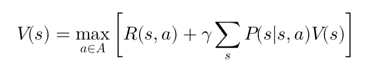
Value Function
The value function, V(s), represents the expected cumulative reward starting from state s and following the optimal policy thereafter. It can be computed using the Bellman equation:
Policy Iteration
Policy iteration is an iterative algorithm used to find the optimal policy. It involves two main steps:
- Policy Evaluation: Calculate the value function for the current policy.
- Policy Improvement: Update the policy by choosing actions that maximize the value function.
This process is repeated until the policy converges to the optimal policy.
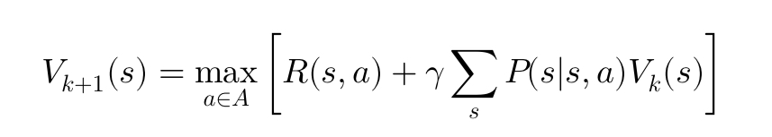
Value Iteration
An alternative to policy iteration is value iteration, which iteratively updates the value function until it converges. The update rule is derived from the Bellman equation:
Applications of MDPs
MDPs are widely used in various fields:
- Robotics: For navigation and manipulation tasks where the robot must make decisions under uncertainty.
- Economics: To model economic decisions and policy making.
- Healthcare: For treatment planning where the outcomes of medical decisions are uncertain.
- Operations Research: For optimizing supply chain and inventory management.
Conclusion
Markov Decision Processes provide a powerful framework for modeling and solving decision-making problems under uncertainty. By understanding the core components and methods of solving MDPs, practitioners can tackle a wide range of complex real-world problems efficiently.