Neural Networks and Deep Learning

Introduction to neural networks

Neural networks are a fundamental concept in the field of artificial intelligence and machine learning. They are computational models inspired by the structure and functioning of biological neural networks in the human brain. Neural networks are composed of interconnected nodes, called neurons or units, organized in layers.

Here’s an introduction to neural networks:

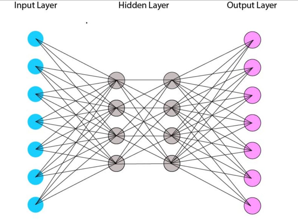
1. Basic Structure: A neural network typically consists of three types of layers: input layer, hidden layers, and output layer. The input layer receives input data, which is then processed through one or more hidden layers containing neurons. Finally, the output layer produces the network’s prediction or output.
2. Neurons (Nodes): Neurons are the building blocks of neural networks. Each neuron receives input signals, applies a transformation function to the inputs, and produces an output signal. Neurons in consecutive layers are connected by weighted connections, which determine the strength of the connections between neurons.
3. Weights and Biases: In neural networks, connections between neurons are associated with weights, which represent the strength of the connection. During training, the network adjusts these weights based on the input data and the desired output. Additionally, each neuron typically has an associated bias, which allows the network to learn more complex patterns.
4. Activation Function: The activation function of a neuron determines its output based on the weighted sum of its inputs. Common activation functions include the sigmoid, tanh (hyperbolic tangent), ReLU (Rectified Linear Unit), and softmax functions. Activation functions introduce non-linearities into the network, enabling it to learn complex patterns and relationships in the data.
5. Training: Training a neural network involves presenting it with a dataset consisting of input-output pairs and adjusting the network’s weights and biases to minimize the difference between the predicted outputs and the true outputs. This process is typically done using optimization algorithms such as gradient descent and its variants, which iteratively update the network’s parameters to minimize a loss function.
6. Backpropagation: Backpropagation is a key algorithm used to train neural networks. It involves computing the gradient of the loss function with respect to the network’s parameters (weights and biases) and using this gradient to update the parameters in the opposite direction of the gradient, thereby minimizing the loss function.
7. Applications: Neural networks have a wide range of applications across various domains, including image recognition, natural language processing, speech recognition, recommender systems, and autonomous vehicles. They have achieved state-of-the-art performance in many tasks, thanks to their ability to learn complex patterns from large datasets.

Overall, neural networks are powerful computational models that have revolutionized machine learning and artificial intelligence. They provide a flexible framework for learning complex patterns and relationships in data, enabling the development of intelligent systems capable of performing a wide range of tasks.

Deep learning architectures

Deep learning architecture is the blueprint of neural networks used in deep learning. These networks consist of layers of interconnected nodes, or neurons, arranged in a hierarchical fashion. Each layer extracts features from the input data and passes them to the next layer for further processing. The architecture defines the arrangement and connections between these layers, which can vary depending on the task and data type. For example, convolutional neural networks (CNNs) are commonly used for image recognition, while recurrent neural networks (RNNs) are suited for sequential data like text or time series. Transformers, another type of architecture, excel in natural language processing tasks. The architecture design plays a crucial role in the network’s ability to learn and generalize from the data, ultimately determining its performance on specific tasks.

Let’s delve into more detail:

1. Convolutional Neural Networks (CNNs): CNNs are specifically designed for tasks involving grid-like data, such as images. They consist of convolutional layers, pooling layers, and fully connected layers. Convolutional layers apply filters (kernels) to the input image to extract features like edges, textures, and patterns. Pooling layers downsample the feature maps to reduce computational complexity. Fully connected layers combine the extracted features and make the final predictions.
2. Recurrent Neural Networks (RNNs): RNNs are suited for sequential data, such as text, speech, or time series. Unlike feedforward neural networks, RNNs have connections that form directed cycles, allowing them to capture temporal dependencies in the data. Each neuron in an RNN receives input not only from the current time step but also from the previous time step, enabling them to maintain a memory of past states.
3. Long Short-Term Memory (LSTM) and Gated Recurrent Unit (GRU): To address the vanishing gradient problem in traditional RNNs, specialized architectures like LSTM and GRU were introduced. These architectures incorporate gating mechanisms that control the flow of information through the network, allowing them to retain information over long sequences and mitigate the issues of vanishing or exploding gradients during training.
4. Transformer Architecture: Transformers have gained prominence in natural language processing (NLP) tasks due to their effectiveness in capturing long-range dependencies in sequences. Unlike RNNs, transformers rely entirely on self-attention mechanisms to weigh the importance of different words in a sentence. They consist of encoder and decoder layers, each composed of multi-head self-attention mechanisms and feedforward neural networks.
5. Autoencoders and Generative Adversarial Networks (GANs): These architectures focus on unsupervised learning and generative modeling. Autoencoders consist of an encoder network that compresses the input data into a latent representation and a decoder network that reconstructs the original data from the latent representation. GANs, on the other hand, consist of a generator network that generates synthetic data samples and a discriminator network that tries to distinguish between real and fake samples. The two networks are trained simultaneously in a competitive fashion, leading to the generation of increasingly realistic samples.

Each of these architectures has its own unique characteristics and applications, and researchers continue to explore new architectures and variations to tackle different types of data and tasks more effectively.

Training deep neural networks

Training deep neural networks involves several key steps and considerations:

1. Data Preparation: Prepare the dataset by cleaning, preprocessing, and splitting it into training, validation, and test sets. Data augmentation techniques may also be applied to increase the diversity of the training data and improve generalization.
2. Model Selection: Choose an appropriate deep learning architecture based on the nature of the data and the task at hand. Consider factors such as the complexity of the problem, the size of the dataset, and computational resources available.
3. Initialization: Initialize the parameters (weights and biases) of the neural network. Common initialization methods include random initialization, Xavier initialization, and He initialization, which help prevent vanishing or exploding gradients during training.
4. Loss Function: Select a suitable loss function that quantifies the difference between the predicted outputs and the true labels. The choice of loss function depends on the type of problem (e.g., classification, regression) and the desired behavior of the model.
5. Optimization Algorithm: Choose an optimization algorithm to update the model parameters during training and minimize the loss function. Popular optimization algorithms include stochastic gradient descent (SGD), Adam, RMSprop, and Adagrad. Each algorithm has its own hyperparameters that need to be tuned for optimal performance.
6. Training Loop: Iterate over the training dataset in mini-batches and perform forward propagation to compute the predicted outputs. Calculate the loss using the chosen loss function and then perform backpropagation to compute the gradients of the loss with respect to the model parameters. Update the parameters using the chosen optimization algorithm.
7. Hyperparameter Tuning: Fine-tune the hyperparameters of the model, such as learning rate, batch size, number of layers, and dropout rate, to optimize performance on the validation set. This process often involves experimentation and iterative refinement to find the best set of hyperparameters.
8. Regularization: Apply regularization techniques such as L1/L2 regularization, dropout, and batch normalization to prevent overfitting and improve the generalization ability of the model.
9. Monitoring and Evaluation: Monitor the training process by tracking metrics such as training loss and validation accuracy. Evaluate the trained model on the test set to assess its performance on unseen data and ensure that it generalizes well.
10. Iterative Improvement: Iterate over the training process, adjusting hyperparameters, trying different architectures, and incorporating feedback from the validation and test sets to iteratively improve the model’s performance.

Training deep neural networks can be computationally intensive and may require significant computational resources, especially for large-scale datasets and complex architectures. Distributed training techniques and specialized hardware accelerators such as GPUs and TPUs can be employed to speed up the training process and handle larger models more efficiently.

Convolutional and recurrent neural networks

Convolutional Neural Networks (CNNs):

1. Architecture:
   • CNNs consist of multiple layers, including convolutional layers, pooling layers, and fully connected layers.
   • Convolutional layers apply filters (kernels) to input data, extracting features like edges, textures, and patterns.
   • Pooling layers downsample feature maps, reducing computational complexity and spatial dimensions.
   • Fully connected layers combine extracted features and make final predictions.
2. Convolution Operation:
   • The convolution operation involves sliding a filter over the input data and computing dot products to produce feature maps.
   • Filters learn to detect specific patterns in the data through the training process.
   • Convolutional layers can have multiple filters to capture different features.
3. Pooling Operation:
   • Pooling layers reduce the spatial dimensions of feature maps while preserving important information.
   • Common pooling operations include max pooling and average pooling.
   • Pooling helps make the model translationally invariant and reduces the number of parameters.
4. Hierarchical Feature Extraction:
   • CNNs learn hierarchical representations of data, with lower layers capturing simple features like edges and higher layers capturing complex features like object parts and shapes.
   • The hierarchical structure allows CNNs to effectively learn features at different levels of abstraction.
5. Applications:
   • CNNs are widely used in computer vision tasks such as image classification, object detection, segmentation, and image generation.
   • They have also been applied to other domains such as natural language processing (e.g., text classification) and speech recognition.

Recurrent Neural Networks (RNNs):

1. Architecture:
   • RNNs are designed to handle sequential data by maintaining a hidden state that captures information from previous time steps.
   • Each neuron in an RNN receives input not only from the current time step but also from the previous time step, allowing it to capture temporal dependencies.
2. Recurrent Connections:
   • Recurrent connections create loops within the network, enabling information to persist over time.
   • RNNs can be unidirectional, where information flows only in one direction, or bidirectional, where information flows in both forward and backward directions.
3. Long Short-Term Memory (LSTM) and Gated Recurrent Unit (GRU):
   • LSTM and GRU are specialized RNN architectures designed to address the vanishing gradient problem and capture long-range dependencies.
   • They incorporate gating mechanisms that control the flow of information through the network, allowing them to retain information over long sequences.
4. Applications
   • RNNs are commonly used in natural language processing tasks such as language modeling, machine translation, sentiment analysis, and speech recognition.
   • They are also applied in time series analysis, including stock market prediction, weather forecasting, and signal processing.
5. Challenges
   • RNNs may suffer from vanishing or exploding gradients during training, which can hinder learning over long sequences.
   • They are also computationally intensive and may struggle with capturing long-range dependencies in very long sequences.
6. Bidirectional RNNs:
   • Bidirectional RNNs combine information from both past and future time steps, allowing them to capture context from both directions and improve performance on tasks like sequence labeling and machine translation.

CNNs and RNNs are powerful architectures that excel in different domains and have their strengths and weaknesses. Researchers often combine these architectures or use variants like Convolutional Recurrent Neural Networks (CRNNs) to leverage the advantages of both for tasks involving sequential and spatial data.