Introduction

Reinforcement Learning (RL) is at the heart of many modern AI applications—robotics, autonomous driving, and game-playing systems like AlphaGo. In RL, an agent interacts with an environment, takes actions, and receives rewards (or penalties) that guide its learning process.

Quantum Reinforcement Learning (QRL) extends this paradigm by leveraging quantum principles like superposition, entanglement, and amplitude amplification. These features allow quantum agents to:

• Explore many possible actions simultaneously,
• Update policies more efficiently, and
• Solve complex decision-making tasks where classical RL is computationally slow.

---

Core Concepts of QRL

1. Quantum States as Policies
   • In classical RL, a policy maps states → actions.
   • In QRL, policies are encoded in parameterized quantum circuits (PQCs), where rotation angles act as weights.
2. Superposition for Exploration
   • Instead of trying actions one by one, the agent evaluates multiple actions in parallel using quantum superposition.
3. Entanglement for Correlation
   • Qubits can be entangled, allowing the agent to model correlated features in the environment naturally.
4. Quantum Measurements as Actions
   • After running the quantum circuit, measurement results collapse into a specific action, chosen with a probability related to the quantum state.

Objective

The goal of this project is to implement a Quantum Reinforcement Learning (QRL) Agent that learns to interact with an environment and maximize rewards using variational quantum circuits (VQCs) as the function approximators.

Instead of relying purely on classical neural networks, QRL leverages quantum superposition and entanglement to represent policies or value functions more efficiently in high-dimensional state spaces.

Example environments:

• CartPole (classic control problem)
• Grid world (toy exploration problem)
• Multi-armed bandit (simplified RL benchmark)

---

Why Quantum RL?

Reinforcement learning is already powerful, but faces challenges:

• Large state-action spaces make classical computation expensive.
• Exploration vs. exploitation trade-off requires efficient representation of uncertainty.
• Scalability: RL agents often need millions of episodes for convergence.

Quantum mechanics offers:

• State encoding via quantum superposition → Compact representation of complex environments.
• Entanglement → Capturing correlations in states and actions.
• Quantum sampling → Faster exploration of possible policies.

---

Core Workflow

1. Environment Setup

• Choose a simple environment (e.g., OpenAI Gym’s CartPole).
• Define states \(s\), actions \(a\), rewards \(r\), and transitions.

2. Quantum Policy Representation

• Use a parameterized quantum circuit (PQC) to represent the policy:

\[πθ(a∣s)=P(action a  ∣  state s,θ)\]

• Encoding: Map classical state \(s\) into a quantum state \(∣ψ(s)⟩\).
• Circuit: Apply parameterized gates \(U(θ)\) that define the policy.
• Measurement: Extract probabilities for choosing each action.

3. Interaction Loop

• The agent takes an action sampled from \(πθ(a∣s)\).
• The environment returns the next state and reward.
• Store transitions \((s,a,r,s’)\).

4. Learning (Classical Optimizer)

• Define a cost function, e.g., expected negative reward or policy gradient objective:

\[J(θ)=E[∑trt]\]

• Use gradient-based classical optimizers (Adam, SGD, SPSA) to update circuit parameters.

5. Training Loop

Repeat until convergence:

1. Encode state into quantum circuit
2. Run circuit → get action probabilities
3. Take action in environment
4. Collect rewards & update PQC parameters

---

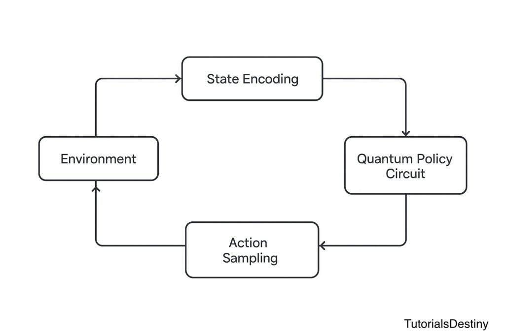
Visual Workflow

Imagine a loop:

Environment → State Encoding → Quantum Policy Circuit → Action Sampling → Environment Feedback → Optimizer Updates Circuit Parameters

---

Mathematical Formulation

Policy Gradient with PQCs

In standard RL, policy gradient is:\[∇θJ(θ)=E[∇θlog⁡πθ(a∣s)⋅R]\]

In QRL:

• \(πθ(a∣s)\) is derived from quantum measurement outcomes.
• The gradient is estimated using the parameter-shift rule:

\[∂∂θ⟨O⟩=12[⟨O⟩θ+π2−⟨O⟩θ−π2]\]

This bridges quantum circuits (policy representation) and classical optimizers (gradient descent).

---

Example Pseudocode

# Initialize quantum policy circuit
policy_qc = VariationalQuantumCircuit(params)

for episode in range(num_episodes):
    state = env.reset()
    total_reward = 0
    
    for step in range(max_steps):
        # Encode state into quantum circuit
        encoded_state = encode_state(state)
        
        # Run circuit to sample action
        action_probs = policy_qc(encoded_state)
        action = sample_action(action_probs)
        
        # Step in environment
        next_state, reward, done, _ = env.step(action)
        
        # Store trajectory
        memory.store(state, action, reward, next_state)
        
        # Update state
        state = next_state
        total_reward += reward
        
        if done:
            break
    
    # Update PQC parameters via classical optimizer
    loss = compute_loss(memory, policy_qc)
    optimizer.step(loss)

print("Training complete")

Frameworks: Qiskit Machine Learning, PennyLane, or Cirq with TensorFlow/PyTorch optimizers.

---

Applications

• Autonomous decision-making in uncertain environments
• Robotics: Navigation & control under uncertainty
• Finance: Optimal portfolio rebalancing using QRL policies
• Quantum chemistry: Adaptive experiments with reinforcement feedback

---

Strengths & Challenges

Strengths

• Compact representation of complex policies
• Natural exploration via quantum randomness
• Potential quantum speedup in policy evaluation

Challenges

• Data encoding bottleneck (quantum feature maps still expensive)
• Hardware noise limits training stability
• Limited number of qubits restricts scalability

---

Project Exercise

• Implement a Quantum Policy Gradient agent for the CartPole environment using PennyLane or Qiskit.
• Compare its training curve with a classical neural network policy.
• Visualize the reward progression (episode vs. reward).
• Reflection: Does QRL converge faster, or does hardware noise slow it down?

---

What’s Next?

➡️ Next: Module 7 – Use Cases & Applications
We will transition from hands-on projects to exploring real-world applications of Quantum AI across drug discovery, finance, natural language processing, and climate modeling.

---