From Learning Everything from Scratch to Reusing Knowledge

Deep learning models are often described as systems that learn from data, but an important question arises when we build a new AI application: does every model really need to learn everything from the beginning?

Imagine training a large neural network to recognize thousands of different objects. Along the way, the network learns edges, shapes, textures, colors, object parts, and complex combinations of these features. Throwing those representations away just because we want to solve a different but related problem would be highly inefficient.

This is where transfer learning becomes valuable. Instead of starting with a randomly initialized network, we take a model that has already learned useful representations from a large dataset and adapt it to a new task. The new model does not begin with an empty slate. It begins with knowledge that has already been learned.

This idea has become one of the most important techniques in modern deep learning, particularly in computer vision and natural language processing.

What Is Transfer Learning?

Transfer learning is the process of taking knowledge learned by a model on one task and reusing it to help solve another related task.

The original problem is called the source task, and the new problem is called the target task. They do not need to be identical. They simply need to share enough useful patterns for the source knowledge to give an advantage on the target.

For example, a network trained on millions of general images learns basic visual structures before progressing to complex shapes. If we now want to identify flower species, training from scratch would force a new network to relearn those basic patterns. With transfer learning, we start from the already-trained network and adapt its visual knowledge to the flower problem.

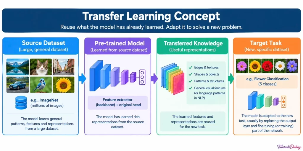
The basic idea can be represented as:

Source Data → Pre-training → Learned Knowledge → Target Data → Adaptation → New Model

The important point is that we are not transferring the original task itself. We are transferring useful knowledge and representations learned during the original training process.

Why Start from a Pre-trained Model?

Training from scratch is perfectly reasonable when we have a huge dataset and need entirely new representations. But it is often impractical. Modern models contain millions or even billions of parameters, and adjusting them demands large amounts of data and computation.

Data is the bigger obstacle. Collecting and labeling it is expensive, especially in specialized fields where every example needs expert review. Imagine building a system that identifies rare plant diseases with only a few thousand specialist-labeled images. Training a large network from scratch on that dataset would likely generalize poorly.

A useful way to think about a pre-trained model is as a student who has already mastered the fundamentals. A student preparing for a specialized engineering exam still has to learn the exam material, but does not need to rediscover arithmetic, algebra, or mathematical reasoning. Likewise, a pre-trained network already contains useful representations, so training can focus on adapting them to the target problem.

Depending on the situation, this can provide several advantages:

• Less training data: useful when the target dataset is small.
• Faster training: much of the representation learning has already been done.
• Lower computational requirements: the whole model may not need training.
• Better initialization: the model starts from meaningful parameters rather than random values.
• Improved performance: especially when the source and target tasks are closely related.

Transfer learning is therefore not just a shortcut. It is a different philosophy of model development: learn useful knowledge once, then reuse it across related problems.

General Features vs Task-Specific Features

To understand why transfer learning works, we need to look at what a network actually learns. It does not simply memorize its training examples. Its parameters are adjusted so that it gradually develops internal representations of patterns in the data, arranged in a hierarchy.

In a convolutional vision network, the hierarchy looks roughly like this:

Early layers
Edges, corners, colors, textures and simple shapes
→ Usually more general

Middle layers
Patterns, structures and object parts
→ Moderately specialized

Deep layers
Complex representations tied to the original task
→ More specialized

Early features are general because they help in many visual tasks. An edge can appear in a car, a building, an animal, or a flower. The deepest layers, by contrast, may be strongly connected to the specific categories the network was originally trained on.

Reuse the general knowledge and adapt the specialized knowledge.

The boundary between general and task-specific knowledge is not fixed, and modern architectures can distribute information in more complicated ways. Still, the hierarchy is a useful guide to which layers we can usually reuse and which we need to adapt.

Pre-training: Learning Before the Final Task

A model is called pre-trained when it has already been trained on a large dataset before being adapted to a particular target task. That original training stage is pre-training.

For a vision model, pre-training may involve millions of images. For a language model, it can involve enormous collections of text. The pre-trained model is not necessarily designed for the exact application we eventually build. Instead, it provides a strong foundation that can later be adapted to a specific problem.

Transfer Learning in Computer Vision

Computer vision offers one of the clearest examples of why transfer learning works. Suppose we want to distinguish several species of flowers using a few thousand labeled images. That sounds like a lot, but it is small relative to the number of parameters in a modern deep network.

A pre-trained vision model has already encountered a far broader collection of images, so its early layers already contain useful detectors for edges, textures, and shapes. We reuse those representations and let the new learning focus on what distinguishes the flower categories. A simplified transfer-learning architecture looks like this:

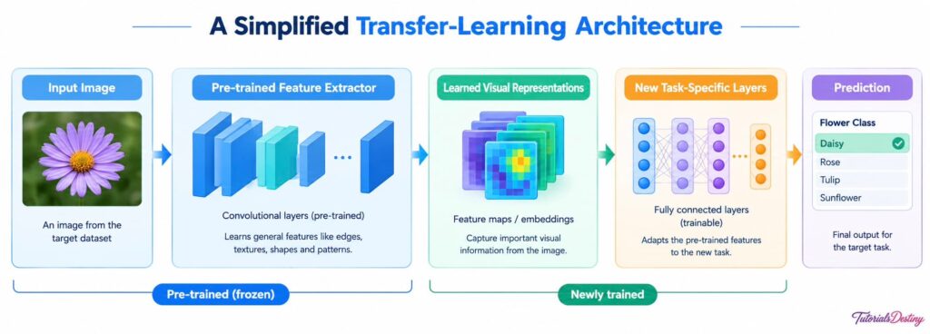
The pre-trained portion provides the foundation, while the new task-specific portion learns to use it for the target problem. The same approach applies to medical image analysis, satellite imagery, industrial inspection, facial recognition, document analysis, object detection, segmentation, and many other vision applications.

Transfer Learning in Natural Language Processing

The same principle becomes even more powerful with language. The meaning of a word depends on its surrounding words, and the meaning of a sentence depends on grammar and broader context. Learning all of this from scratch for every NLP application would be extremely inefficient.

Instead, a language model is first pre-trained on a very large collection of text. It develops broad representations of vocabulary, syntax, sentence structure, context, and meaning, without being tied to one narrow task. Afterwards it can be adapted to tasks such as:

• sentiment analysis,
• named entity recognition,
• text classification,
• question answering,
• summarization,
• language generation, and conversational applications.

Take customer-review sentiment analysis. The pre-trained model knows a great deal about English but does not know which language patterns count as positive, negative, or neutral for our application. We add a small task-specific classification component, train it on a labeled sentiment dataset, and, if needed, fine-tune parts of the language model itself. The data has changed from images to text, but the process is the same:

Learn broadly first, specialize later.

Feature Extraction and Fine-Tuning

Two Ways to Reuse a Pre-trained Network

The practical question is how to use a pre-trained model’s knowledge. We could use it exactly as it is, but its original output layer may not match our problem. We could retrain everything, but that would throw away much of the advantage. In practice, transfer learning is a balance between preserving what the model already knows and allowing it to learn what is new. Two approaches dominate:

1. Feature extraction — keep the pre-trained network fixed and use its learned representations for the new task.
2. Fine-tuning — allow some pre-trained layers to keep learning so the model adapts more closely to the target dataset.

Feature Extraction: Using What the Model Already Knows

Feature extraction is the more conservative approach. The pre-trained network already transforms an input into a rich internal representation, so instead of changing it, we use it as a feature extractor and attach a new task-specific layer, or a small group of layers, at the end. Only the new layers are trained:

Input Image → Pre-trained Layers (Frozen) → Learned Feature Representation → New Classification Head (Trainable) → Target Prediction

A general image model may already understand shapes, textures, and object structures. For flower classification, the new head simply learns which combinations of those features correspond to each flower category.

Why Freeze the Pre-trained Layers?

A frozen layer is one whose parameters are not updated during the new training. Normally, training computes gradients and uses them to update every parameter; a frozen layer skips that step, so its learned knowledge stays intact while the trainable layers adapt.

Freezing helps for two reasons. First, a small dataset cannot safely guide the modification of millions of parameters; the network may adapt too closely to the training examples, which is overfitting. Freezing greatly reduces the number of parameters to learn. Second, fewer trainable parameters mean a simpler, cheaper optimization problem. Feature extraction is therefore especially attractive when the target dataset is small and reasonably similar to the pre-training data.

The Classification Head: Where the New Task Lives

It helps to think of a network as two parts: feature extractor + task-specific head. The extractor turns raw input into meaningful representations. The head turns those representations into the final prediction.

Suppose the original model classifies 1,000 object categories but our application needs only five flower types. The original output layer is built for 1,000 classes, so we remove it and attach a new five-class head. The rest of the network stays largely unchanged. This is one of the simplest and most common forms of transfer learning, and the same idea applies beyond classification: the head is always rebuilt to match whatever the new task requires.

This is also why transfer learning focuses on representations rather than predictions. A model that outputs “Dog: 92%, Cat: 5%, Fox: 2%” has final predictions tied to its original task, but somewhere inside it holds a rich description of shapes, textures, and body structures that can be reused for entirely new categories.

Fine-Tuning: Teaching the Model About the New Domain

Feature extraction assumes the pre-trained representations are already good enough. When the new task differs more, they may need adjustment. Fine-tuning means allowing some of the pre-trained parameters to be updated using the target dataset. The model still starts from its pre-trained knowledge, but we make controlled adjustments to suit the new problem.

For example, a model trained mainly on everyday photographs may be adapted to spot abnormalities in medical scans. Some visual patterns remain useful, but the deeper representations may need to capture structures that never mattered during the original training. Fine-tuning makes those adjustments without discarding the entire pre-trained representation.

It is also not simply “training again”. When training from scratch, a network learns fundamental representations for the first time. During fine-tuning, it already contains substantial learned structure, and the goal is specialization: refining what the model already knows.

Freezing and Unfreezing: Which Layers to Train

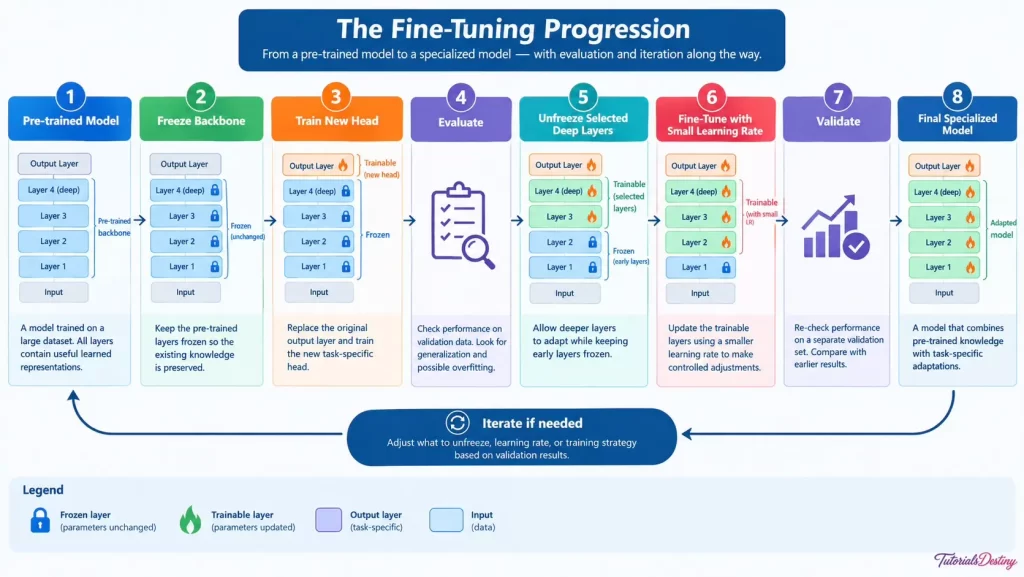
Fine-tuning does not mean retraining every layer. Following the feature hierarchy described earlier, we usually leave the early, general layers frozen and unfreeze the deeper, more specialized ones first, gradually moving backward through the network:

Task-specific head → deeper layers → possibly middle layers

This protects the useful low-level representations. How much to unfreeze has no universal answer; it depends on dataset size and on how different the target domain is. A small, similar dataset may only need the new head trained. A larger or more different dataset may benefit from several deeper blocks being fine-tuned.

This gives a natural two-stage strategy:

Stage 1: backbone frozen, new head trainable → learn the new task on stable representations.

Stage 2: earlier layers frozen, selected deeper layers and head trainable → fine-tune with a small learning rate.

This is usually more stable than unfreezing the whole network immediately. The practical mindset is: start conservatively, measure the result, and increase adaptation only when the evidence supports it.

Why Fine-Tuning Uses a Smaller Learning Rate

When training from scratch, parameters start random and need large adjustments. During fine-tuning, the model already contains useful knowledge, and large updates could overwrite it after only a few training steps. For this reason, fine-tuning commonly uses a smaller learning rate than training from scratch.

The basic parameter-update equation is:

$\theta_{\text{new}} = \theta_{\text{old}} – \eta\nabla_{\theta}L$

where:

• $\theta$ represents the model parameters,
• $\eta$ represents the learning rate,
• $L$ represents the loss function,
• $\nabla_{\theta}L$ represents the gradient of the loss with respect to the parameters.

A smaller $\eta$ acts like a form of caution. The model is essentially being told: “You already know a lot. Make careful adjustments rather than completely changing what you have learned.” This matters most when the target dataset is small.

Discriminative (layer-wise) learning rates. Different parts of the network can use different rates. The newly created head has no useful pre-trained knowledge and needs the most learning, while the early layers hold the most reusable knowledge and should change least:

• Early layers → very small learning rate
• Middle layers → small learning rate
• Task-specific head → comparatively larger learning rate

Catastrophic Forgetting

One risk of aggressive fine-tuning is catastrophic forgetting: the model learns the new task but loses important knowledge it had previously acquired. If a network with strong general representations is pushed hard on a small, very different dataset, it may excel on the target training data while losing the broader features that made it useful in the first place.

Low learning rates, frozen early layers, and gradually increasing the number of trainable layers all reduce this risk. The broader principle: learning something new should not require forgetting everything learned before.

Recognizing Overfitting During Fine-Tuning

Fine-tuning brings back a familiar problem: overfitting. Suppose training accuracy keeps climbing while validation accuracy stalls or drops:

Training accuracy: 92% → 95% → 98%
Validation accuracy: 90% → 91% → 87%

The model is learning the training data extremely well, but its ability to generalize to unseen images is getting worse. Higher training accuracy does not necessarily mean a better model. Several techniques help:

• data augmentation,
• regularization and dropout,
• fewer trainable layers,
• a lower learning rate,
• early stopping, and careful monitoring of validation performance.

Data augmentation deserves a special mention. In vision, it creates modified versions of existing images through rotation, cropping, flipping, scaling, or brightness changes. The goal is not just more images but exposure to reasonable variations: a slightly rotated flower should remain the same class. Combined with transfer learning, this makes a small dataset go much further, provided the transformations reflect realistic variations in the target domain.

Choosing Between Feature Extraction and Fine-Tuning

Both approaches reuse a pre-trained model, but they suit different situations.

Feature Extraction	Fine-Tuning
Pre-trained layers remain frozen	Some pre-trained layers are updated
Only new task-specific layers are trained	New layers and selected existing layers are trained
Lower computational cost	Higher computational cost
Useful with smaller datasets	Often useful when more target data is available
Lower risk of damaging learned representations	Greater ability to adapt to the target domain
Good when source and target domains are similar	Useful when the target domain differs more significantly

A simple decision guide, starting from the target dataset:

• Small dataset + similar domain → start with feature extraction.
• Moderate dataset + related domain → feature extraction, then selective fine-tuning.
• Larger dataset + significant domain difference → more extensive fine-tuning.
• Very different domain → carefully evaluate whether the pre-trained model is appropriate at all.

This is a starting point, not a rigid formula; it should always be validated experimentally. The choice is also not permanent. A common workflow begins with feature extraction, and only if performance is insufficient are selected layers unfrozen. A small dataset does not rule out fine-tuning either; it just means fine-tuning must be done carefully. Throughout, the objective is not to change as much as possible but to change just enough.

Source and Target Domains

One of the biggest factors in transfer learning is how the source and target domains relate. A model trained on everyday photographs is a strong starting point for classifying animals, but a weaker one for specialized medical imaging, whose structures and textures differ. It would be useless for numerical financial records, however powerful the model is. In general:

The greater the similarity between source and target, the less adaptation is needed. The greater the difference, the more carefully we should consider fine-tuning.

Domains need not be identical, and knowledge sometimes transfers across surprisingly different tasks. Transfer learning is a spectrum, and the real questions are how much knowledge to transfer, which to preserve, and which to adapt.

Domain shift occurs when the statistical characteristics of the target data differ from the source data. A model trained on high-quality studio photographs may struggle on low-light security-camera footage: the objects are similar, but lighting, resolution, angle, background, and noise have changed. Domain shift can also come from different populations, writing styles, languages, sensors, or data-collection methods, so the model must be evaluated on data that realistically represents its final environment. Methods for handling the gap are called domain adaptation.

Negative transfer is the worst case: the transferred knowledge makes target performance worse than it would have been without it. It can happen when domains are too different or the representations are poorly suited to the target.

The safeguard is a baseline. A result like 91% validation accuracy means little in isolation: against a baseline of 89% the gain is modest, against 65% it is major. A good experiment compares a model trained from scratch, feature extraction, and fine-tuning, and asks not “should fine-tuning work better?” but “does fine-tuning actually improve performance on our validation set?”

Choosing a Pre-trained Model

A pre-trained model is not automatically useful because it is large, popular, or accurate on its original benchmark. Choosing one is an engineering decision with several dimensions.

• The task: start by asking what the target application actually requires. A classification model suits classification, while locating multiple objects needs an architecture that preserves spatial information.
• The architecture: convolutional networks and Vision Transformers extract image information differently, and Transformers have become central in NLP because attention captures relationships across a sequence. The architecture should fit the structure of the problem.
• The pre-training dataset: a model trained on data close to your domain, such as medical scans or satellite imagery, may offer a stronger starting point than one trained on ordinary photographs. Biases or limitations in the source data can also be inherited by the adapted model.
• Size and deployment: larger models have more capacity but need more memory, computation, and time. A model that runs on a modest machine may beat a slightly more accurate one that needs a powerful GPU, especially on mobile or edge devices.
• More than accuracy: inference speed, latency, memory, energy use, reliability, and scalability all matter. An autonomous system that must predict in milliseconds cannot use a slow model, however accurate.

The best model is not always the largest. It is the one that best balances performance, efficiency, cost, and complexity for your problem. Ask not only “Is this model powerful?” but “Is this model appropriate for my data, my task, and my constraints?”

A Real-World Transfer Learning Workflow

Now let us bring these decisions together in one realistic project: an image classification system that identifies five types of flowers. The same workflow applies to industrial inspection, medical imaging, agriculture, wildlife monitoring, and document analysis.

1. Define the target problem. The input is an image and the output is one of five classes. This determines the final layer, the loss function, and the evaluation metrics. It also includes the deployment environment: if the model will receive phone photos with shadows, cluttered backgrounds, and varied lighting, studio-only training images will leave it struggling after deployment.

2. Prepare the target dataset. Gather correctly labeled examples with real variation in orientation, lighting, background, size, and growth stage. Transfer learning cannot compensate for systematically wrong labels. Then split the data into three sets:

• Training set — used to update the trainable parameters.
• Validation set — used to monitor performance during development.
• Test set — used only for final evaluation.

Keeping these roles separate matters: reusing the same images to make decisions and then report final performance makes the results overly optimistic.

3. Choose a pre-trained model. For flowers, a vision model pre-trained on a broad collection of natural images is a sensible fit, since its early layers provide general visual features and its deeper layers hold useful knowledge about natural structures. Weigh the factors from the previous section, such as architecture, size, and deployment needs.

4. Replace the output layer. Swap the original 1,000-class head for a new five-class head:

Input Image → Pre-trained Backbone → Feature Representation → New Five-Class Output Layer → Flower Prediction

5. Start with feature extraction. Freeze the backbone and train only the new head. The model is effectively asking: “Given the features the pre-trained model already produces, how can I use them to distinguish these five categories?” If the domains are related, it may already perform surprisingly well.

6. Evaluate. If validation performance is strong and stable, there may be no reason to fine-tune at all; fine-tuning should not be performed just because it is available. If performance plateaus below what the application needs, the representations are probably useful but not perfectly adapted, and fine-tuning is worth investigating.

7. Unfreeze gradually and fine-tune. Unfreeze one deeper block, fine-tune with a small learning rate, evaluate again, and repeat only if the evidence supports it. If a step makes validation performance worse, reconsider how much of the network should be trainable, and watch for the overfitting pattern described earlier.

8. Evaluate on the test set. Finally, measure performance on data that was never used for training or model selection. This gives a realistic estimate of how the model will behave on new images.

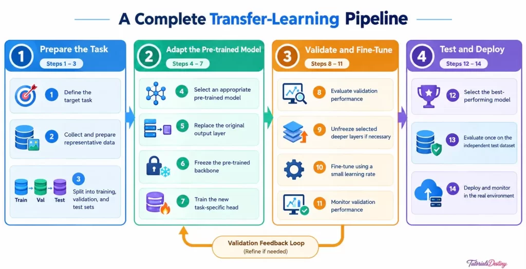
The pipeline captures the central philosophy of transfer learning: start with existing knowledge, preserve what is useful, adapt what is necessary, and continuously validate whether the adaptation is actually helping.

The flower example is friendly because general image features suit another image task. With a very different target, such as medical imaging, replacing the head will not be enough; expect more extensive fine-tuning, stronger preprocessing, domain-specific augmentation, and careful validation.

From Transfer Learning to Foundation Models

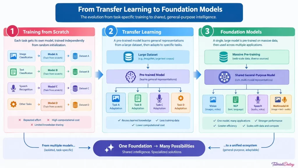
Transfer learning changed how AI systems are built. In a traditional workflow, each problem got its own model, trained on its own dataset. Deep learning moved toward a different pattern:

Large-scale pre-training → reusable knowledge → task-specific adaptation

One large model can be trained once and become the foundation for many applications. This reduces the labeled data needed, shortens development time, and makes advanced AI more accessible, since adapting an existing model is far more practical than training a massive one from scratch.

Today’s foundation models extend this idea: they are trained on very large and diverse datasets as general-purpose bases for many downstream tasks. Large language models are the most visible example, but the same philosophy now appears in computer vision, speech, and multimodal AI. The difference from classic transfer learning is mainly one of scale.

As models grew, fine-tuning every parameter became expensive. Maintaining a separate fully fine-tuned copy of a billion-parameter model for every application takes substantial storage and computation. This motivated parameter-efficient fine-tuning (PEFT), which keeps most pre-trained parameters unchanged and trains only a much smaller set. One important example is Low-Rank Adaptation (LoRA), which learns a small adaptation to the model’s weights instead of rewriting them for every task.

The principle is the same as in classical transfer learning: preserve the expensive knowledge, and change only what needs to change.

Key Takeaways

Transfer learning lets a network trained on one task or dataset provide useful knowledge for another related task, so the new model does not have to learn every representation from the beginning.

Feature extraction is the conservative option: freeze the pre-trained backbone and train a new task-specific head. Fine-tuning goes further by letting selected deeper layers adapt, which helps when the target domain differs from the source or feature extraction plateaus.

The most successful workflows are controlled rather than aggressive: train the new head, evaluate, and fine-tune only when the evidence says it will help, using small learning rates and watching validation performance for overfitting. Throughout, compare against a baseline rather than assuming transfer will help.

The same ideas now underpin parameter-efficient adaptation and foundation-model workflows, where enormous pre-trained models are reused across many applications.

Learning builds knowledge.
Transfer learning reuses knowledge.
Fine-tuning specializes knowledge.

What Comes Next: Natural Language Processing

Language poses a different challenge from images. Images have spatial relationships between pixels, while language has relationships between words, phrases, and sentences, often across long distances. CNNs showed how networks learn hierarchical spatial representations, RNNs showed how they process sequences, and transfer learning showed how learned representations can be reused.

Natural Language Processing will explore how AI systems process, represent, understand, and generate human language. That journey begins with the foundations of text processing: how raw language is transformed into a form that a machine-learning model can actually understand.