Measuring Machine Learning Success

Building a Machine Learning model is an exciting achievement, but creating a model is only half of the journey. A model that appears impressive during development may completely fail when deployed in the real world. For this reason, evaluating model performance is one of the most important stages of the Machine Learning lifecycle.

Imagine a hospital implementing an AI system to detect cancer. The model reports an accuracy of 98%, which initially sounds excellent. However, further investigation reveals that it misses many actual cancer cases. Despite its high accuracy, the model is not reliable enough for healthcare applications.

Now consider a fraud detection system used by a bank. The system successfully identifies fraudulent transactions but also incorrectly flags thousands of legitimate transactions every day. While it catches fraud, it creates frustration for customers and increases operational costs.

These examples demonstrate a crucial principle:

A Machine Learning model should not be judged by a single number alone.

Developers need a comprehensive understanding of how a model behaves, where it succeeds, and where it fails. This is the purpose of model evaluation.

In this lesson, we will explore the techniques used to measure Machine Learning performance and learn how evaluation helps organizations deploy reliable AI systems.

Why Evaluation Matters in Real-World AI Systems

Artificial Intelligence increasingly influences decisions that affect people’s lives. AI systems recommend products, approve loans, diagnose diseases, identify security threats, and even assist autonomous vehicles.

In such environments, incorrect predictions can have significant consequences.

A recommendation system that suggests an irrelevant movie may be inconvenient but harmless. A medical diagnosis system that fails to detect a serious illness can have far greater consequences.

This means developers must answer several important questions before deploying a model:

• How accurate is the model?
• How often does it make mistakes?
• What kinds of mistakes does it make?
• Can it generalize to new data?
• Is it suitable for real-world use?

Without proper evaluation, these questions remain unanswered.

Evaluation provides evidence that a model is performing as expected and helps identify weaknesses before deployment.

The Cost of Incorrect Predictions

Not all prediction errors have the same impact.

Some mistakes may be relatively harmless, while others can be extremely costly.

Understanding the consequences of incorrect predictions helps us appreciate why evaluation metrics are so important.

Example: Email Spam Detection

Suppose an email system incorrectly labels a legitimate message as spam.The user may miss an important email, causing inconvenience.

Now consider the opposite scenario.

The system fails to identify a spam email. The user receives an unwanted message.

Both outcomes are undesirable, but organizations may prefer one type of error over the other depending on their priorities.

Example: Medical Diagnosis

Consider a disease detection system.

If the model predicts that a healthy patient is sick, additional testing may be required. This is inconvenient but often manageable.

However, if the model predicts that a sick patient is healthy, treatment may be delayed.

This error could have serious consequences.

Example: Fraud Detection

A bank uses Machine Learning to detect fraudulent transactions.

If the model incorrectly blocks a legitimate transaction, customers may become frustrated.

If the model misses actual fraud, the bank may lose money.

Both errors are costly but affect the business differently.

These examples illustrate why Machine Learning evaluation goes beyond simple accuracy measurements.

Understanding the types of errors a model makes is often more important than knowing how many predictions are correct.

The Foundation of Reliable Evaluation

Before measuring performance, developers must ensure that evaluation is performed fairly.

Evaluating a model using the same data that was used for training creates misleading results.

The model may simply memorize the training examples.

To prevent this problem, Machine Learning datasets are usually divided into separate subsets.

Training Data

Training data is used to teach the model.

During training, the algorithm learns patterns and relationships from examples.

For example, a house price prediction model may learn how factors such as:

• House size
• Number of bedrooms
• Location
• Property age

influence property values.

The model adjusts its internal parameters until it can make increasingly accurate predictions.

Training data serves as the learning material for the algorithm.

Validation Data

Validation data is used during development.

The model does not learn directly from validation data.

Instead, developers use it to:

• Compare different models
• Tune hyperparameters
• Detect overfitting
• Improve performance

Validation data acts as a checkpoint during the development process.

It helps developers make informed decisions before final testing.

Test Data

The test dataset is used after training is complete.

Its purpose is to provide an unbiased assessment of model performance.

The model has never seen this data before.

As a result, testing provides a realistic estimate of how well the system will perform in real-world situations.

A model that performs well on testing data is more likely to generalize successfully.

Understanding Generalization

One of the primary goals of Machine Learning is generalization.

Generalization refers to a model’s ability to perform well on new, unseen data.

A model that memorizes training examples may achieve excellent training accuracy but poor real-world performance.

Conversely, a model that learns underlying patterns can adapt to unfamiliar situations.

Consider a student preparing for an examination. A student who memorizes answers may perform well if the same questions appear.

A student who understands concepts can answer new questions as well.

Machine Learning models behave in a similar manner. The goal is not memorization. The goal is understanding patterns. Evaluation helps determine whether a model has truly learned or simply memorized.

Understanding Prediction Outcomes

To evaluate Machine Learning models effectively, we must understand the possible outcomes of a prediction.

Consider a disease detection system. The model predicts whether a patient has a disease.

Four outcomes are possible.

True Positive (TP)

The patient has the disease. The model correctly predicts the disease. This is a correct positive prediction.

True Negative (TN)

The patient does not have the disease. The model correctly predicts no disease. This is a correct negative prediction.

False Positive (FP)

The patient is healthy. The model incorrectly predicts disease. This is sometimes called a “false alarm.”

False Negative (FN)

The patient has the disease. The model incorrectly predicts no disease. This is often the most dangerous type of error in healthcare applications.

Why Prediction Outcomes Matter

These four outcomes form the foundation of nearly every evaluation metric used in Machine Learning.

Without understanding these categories, it becomes impossible to interpret performance measurements correctly.

For example:

• Accuracy depends on correct predictions.
• Precision depends on true positives and false positives.
• Recall depends on true positives and false negatives.

Every classification metric ultimately builds upon these four outcomes.

The Confusion Matrix

The confusion matrix is one of the most valuable tools in Machine Learning evaluation. It provides a structured summary of prediction outcomes.

A typical confusion matrix looks like this:

	Predicted Positive	Predicted Negative
Actual Positive	✅ (TP)	❌ (FN)
Actual Negative	❌ (FP)	✅ (TN)

This table allows developers to see exactly how the model performs. Rather than simply reporting accuracy, the confusion matrix reveals where errors occur.

A Practical Confusion Matrix Example

Suppose a disease detection system evaluates 1,000 patients.

The results are:

	Predicted Positive	Predicted Negative
Actual Positive	✅ 80 (TP)	❌ 20 (FN)
Actual Negative	❌ 10 (FP)	✅ 890 (TN)

This means:

• 80 sick patients were correctly identified.
• 20 sick patients were missed.
• 10 healthy patients were incorrectly flagged.
• 890 healthy patients were correctly identified.

This single table provides far more insight than an accuracy percentage alone.

What We Can Learn from the Confusion Matrix

The confusion matrix helps answer important questions:

• How many positive cases were detected?
• How many cases were missed?
• How often are false alarms occurring?
• Which type of error is more common?

Different applications may prioritize different outcomes.

For example:

Healthcare: Reducing false negatives is often critical.

Cybersecurity: Reducing missed attacks is essential.

Marketing: Reducing false positives may be more important.

The confusion matrix provides the information needed to make these decisions.

Classification Metrics: Looking Beyond Accuracy

When beginners first learn Machine Learning, accuracy is usually the first metric they encounter. Accuracy is useful because it is easy to understand. However, it often fails to tell the full story.

Consider a fraud detection system:

• 9,900 legitimate transactions
• 100 fraudulent transactions

Suppose the model predicts every transaction as legitimate.

The result:

• 9,900 correct predictions
• 100 incorrect predictions

The model achieves: 90.9%? No.

It actually achieves: 99% accuracy.

Despite this impressive number, the model fails to detect any fraud.

Clearly, accuracy alone is insufficient. This is why Machine Learning practitioners rely on multiple evaluation metrics.

Accuracy: The Most Familiar Metric

Accuracy measures the proportion of correct predictions.

The formula is:

$Accuracy=\frac{TP+TN}{TP+TN+FP+FN}$

Accuracy provides a simple overview of performance.

For example:

If a model makes 1,000 predictions and 950 are correct:

Accuracy = 95%

This means the model correctly predicts outcomes 95% of the time.

Advantages of Accuracy

Accuracy offers several benefits:

• Easy to calculate
• Easy to understand
• Useful for balanced datasets
• Widely recognized

Because of its simplicity, accuracy is often used as an initial performance indicator.

Limitations of Accuracy

Accuracy can become misleading when:

• Classes are imbalanced
• Certain errors are more costly
• Rare events are important

For example:

• Fraud detection
• Medical diagnosis
• Cybersecurity

In these situations, additional metrics are required.

When Should Accuracy Be Used?

Accuracy works best when:

• Classes are balanced
• All errors have similar costs
• Prediction categories occur with similar frequency

Examples include:

• Basic image classification
• Product categorization
• Document classification

Even in these cases, experienced practitioners often use additional metrics for deeper analysis.

Precision: Measuring Prediction Quality

Suppose an email system identifies messages as spam.

The model flags 100 emails as spam.

Out of those 100 emails:

• 90 are actually spam
• 10 are legitimate messages

Precision measures how many positive predictions were correct.

Precision answers:

When the model predicts a positive outcome, how often is it right?

A high precision score means the model produces fewer false alarms. This is especially important when false positives are costly.

When Precision Matters Most

Precision is particularly important in applications such as:

• Email Filtering: Legitimate emails should not be incorrectly marked as spam.
• Fraud Detection: Customers should not have their valid transactions blocked unnecessarily.
• Legal Document Analysis: Incorrect classifications can create costly consequences.

In such situations, organizations often prioritize precision over recall.

Calculating Precision

The precision formula is:

$Precision=\frac{TP}{TP+FP}$

A higher precision score indicates better prediction quality. However, precision alone does not tell the complete story.

Recall: Measuring Detection Capability

Precision focuses on the quality of positive predictions. However, a model can achieve high precision simply by being extremely selective about when it predicts a positive outcome.

This raises an important question:

How many actual positive cases is the model successfully identifying?

This is where recall becomes important. Recall measures a model’s ability to find all relevant positive cases within a dataset.

In simple terms, recall answers:

Out of all the actual positive cases, how many did the model correctly identify? A model with high recall successfully detects most positive examples and minimizes missed cases.

Understanding Recall Through a Medical Example

Imagine a hospital develops an AI system to detect cancer.

Suppose:

• 100 patients actually have cancer.
• The model correctly identifies 90 patients.
• The model misses 10 patients.

In this scenario:

• True Positives = 90
• False Negatives = 10

The recall is:

90 ÷ (90 + 10)= 90%

This means the model successfully detected 90% of all cancer cases.

Why Recall Matters

Recall becomes critical whenever missing a positive case could have serious consequences.

Examples include:

Medical Diagnosis: Missing a disease diagnosis may delay treatment.

Fraud Detection: Undetected fraudulent transactions can result in financial losses.

Cybersecurity: Missing a security breach can expose an organization to significant risk.

Disaster Prediction: Failure to identify dangerous conditions can threaten public safety.

In these situations, organizations often prioritize recall over precision.

Calculating Recall

Recall is calculated using:

$Recall=\frac{TP}{TP+FN}$

A high recall score indicates that the model successfully identifies most positive cases. However, maximizing recall alone can create new challenges.

Precision vs Recall: Understanding the Tradeoff

One of the most important concepts in Machine Learning evaluation is the relationship between precision and recall. Improving one metric often reduces the other.

Consider an email spam filter.

Strategy 1: Maximize Precision

The model only labels emails as spam when it is almost completely certain.

Result:

• Very few legitimate emails are incorrectly flagged.
• Some spam emails are missed.

Precision increases.

Recall decreases.

Strategy 2: Maximize Recall

The model aggressively labels suspicious emails as spam.

Result:

• Most spam messages are caught.
• More legitimate emails are incorrectly flagged.

Recall increases.

Precision decreases.

Visualizing the Precision-Recall Tradeoff

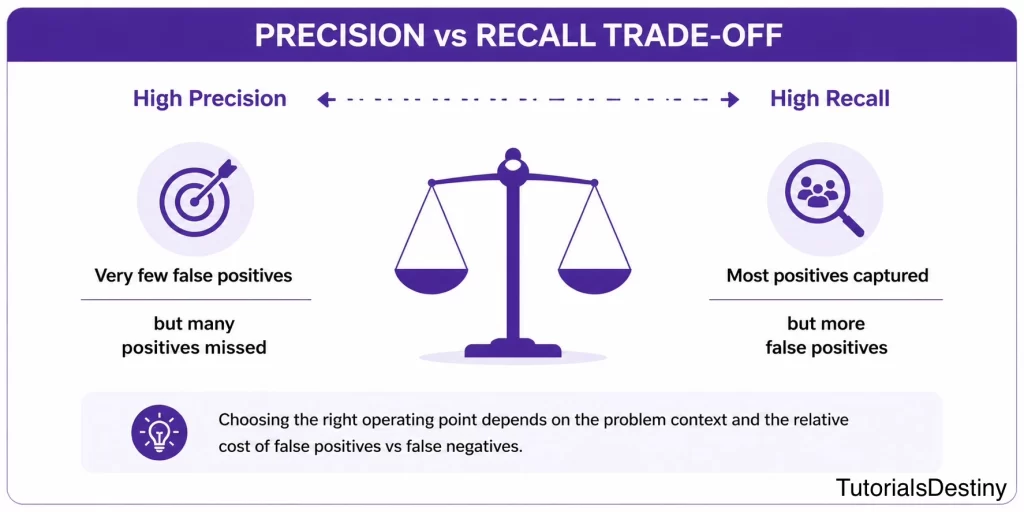
Finding the ideal balance depends on the business problem.

Choosing Between Precision and Recall

Different applications prioritize different objectives.

Application	Priority
Cancer Detection	Recall
Fraud Detection	Balance
Email Spam Filtering	Precision
Security Monitoring	Recall
Recommendation Systems	Balance

Understanding business requirements is essential when selecting evaluation metrics.

F1 Score: Balancing Precision and Recall

Since precision and recall often compete with one another, Machine Learning practitioners frequently use a metric that combines both. This metric is called the F1 Score. The F1 Score calculates the harmonic mean of precision and recall.

Rather than favoring one metric over the other, it rewards models that perform well on both.

Why the F1 Score Exists

Suppose two models achieve the following results:

Model A

• Precision = 95%
• Recall = 40%

Model B

• Precision = 85%
• Recall = 85%

Although Model A has excellent precision, it misses many positive cases. Model B provides a better overall balance.

The F1 Score helps identify this difference.

Calculating the F1 Score

$F1=2\times\frac{Precision\times Recall}{Precision+Recall}$

The score ranges between:

• 0 = Poor performance
• 1 = Perfect performance

Higher values indicate stronger overall classification performance.

When Should You Use F1 Score?

The F1 Score is particularly useful when:

• Datasets are imbalanced.
• Both false positives and false negatives matter.
• Accuracy is misleading.
• Precision and recall are equally important.

Its applications includes Fraud detection, Medical diagnosis, Information retrieval and Natural Language Processing

Understanding Classification Thresholds

Many Machine Learning models do not directly predict categories. Instead, they generate probabilities.

For example:

Customer	Purchase Probability
A	0.95
B	0.78
C	0.52
D	0.40

Developers must choose a threshold that determines when a prediction becomes positive.

The Default Threshold

A common threshold is: 0.5

This means:

• Probability ≥ 0.5 → Positive
• Probability < 0.5 → Negative

However, this threshold is not always optimal.

How Thresholds Affect Performance

Suppose we lower the threshold.

Instead of requiring 0.5, we require only 0.3.

The model becomes more willing to predict positive outcomes.

Result:

• Recall increases.
• Precision may decrease.

Now suppose we raise the threshold to 0.8.

The model becomes more selective.

Result:

• Precision increases.
• Recall decreases.

This demonstrates why threshold selection is important.

Real-World Threshold Example

Consider fraud detection.

A bank may decide:

• 0.90 probability → Automatically block transaction.
• 0.70 probability → Request verification.
• Below 0.70 → Allow transaction.

Different thresholds create different business outcomes.

Evaluation helps organizations choose appropriate values.

ROC Curves: Evaluating Performance Across Thresholds

Changing thresholds affects model performance. Instead of evaluating only one threshold, we can evaluate many.

The Receiver Operating Characteristic (ROC) Curve helps visualize performance across different threshold settings.

The ROC curve compares:

• True Positive Rate
• False Positive Rate

at multiple thresholds.

Understanding the ROC Curve

A ROC curve generally looks like:

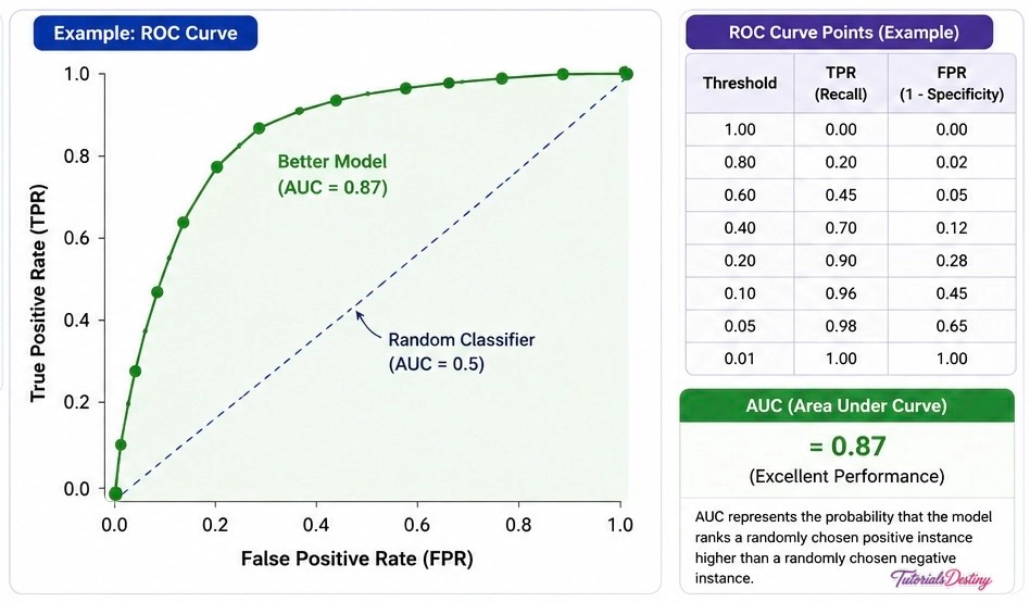
Better models push the curve closer to the upper-left corner.

Interpreting ROC Curves

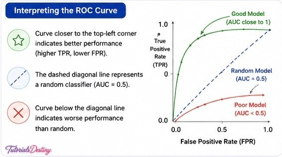
Upper Left Corner

Represents excellent performance, High detection rate and Low false alarms.

Diagonal Line

Represents random guessing. The model performs no better than chance.

Below the Diagonal

Indicates poor performance and predictions are often incorrect.

Area Under the Curve (AUC)

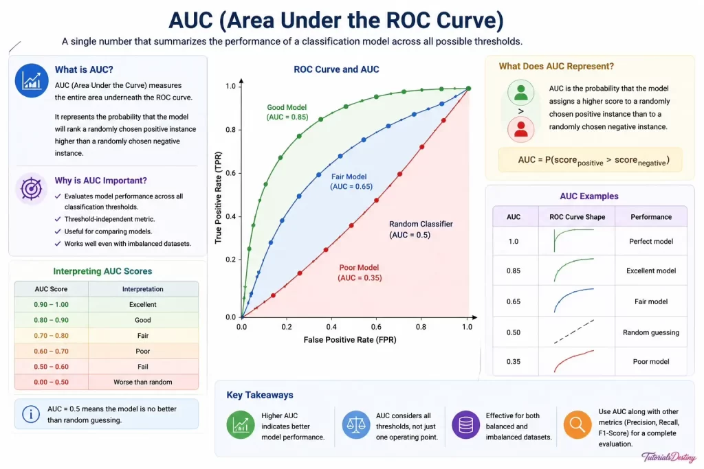
Rather than analyzing the entire ROC curve, we often calculate a single summary value.

This value is called AUC.

AUC stands for: Area Under the ROC Curve.

Interpreting AUC Scores

AUC Score	Performance
0.30	Poor Model
0.50	Random Guessing
0.65	Fair Model
0.85	Excellent Model
1.0	Perfect Model

Higher values indicate stronger classification performance.

Why ROC-AUC Is Popular

ROC-AUC provides several advantages:

• Independent of a specific threshold
• Easy model comparison
• Effective overall performance measure
• Widely used in industry

Many Machine Learning competitions use ROC-AUC as a primary evaluation metric.

Precision-Recall Curves

Although ROC curves are useful, they may sometimes be misleading.

This is especially true when datasets are highly imbalanced.

Consider:

• 99,000 normal transactions
• 1,000 fraudulent transactions

Even poor models may achieve impressive ROC scores.

In such situations, Precision-Recall (PR) Curves often provide more meaningful insights.

Understanding Precision-Recall Curves

A Precision-Recall Curve plots:

• Precision
• Recall

across different thresholds.

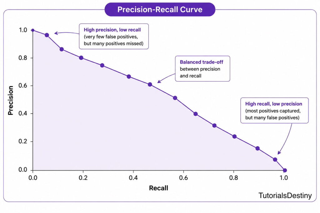
The shape of the curve illustrates how precision changes as recall increases.

When Precision-Recall Curves Are Preferred

PR Curves are particularly useful for:

• Fraud detection
• Rare disease detection
• Cybersecurity
• Anomaly detection

Whenever positive cases are rare, Precision-Recall analysis often provides a clearer picture of model performance.

Comparing ROC and Precision-Recall Curves

ROC Curve	Precision-Recall Curve
Uses TPR and FPR	Uses Precision and Recall
Works well on balanced datasets	Better for imbalanced datasets
Widely used	More informative for rare events
Evaluates ranking quality	Focuses on positive class performance

Professional Machine Learning practitioners often examine both.

Key Takeaways

• Recall measures how many positive cases are successfully detected.
• Precision and recall often compete with one another.
• F1 Score balances precision and recall.
• Classification thresholds influence model behavior.
• ROC Curves evaluate performance across thresholds.
• AUC summarizes ROC performance.
• Precision-Recall Curves provide valuable insight for imbalanced datasets.
• Different evaluation metrics serve different business objectives.

Regression Evaluation Metrics: Measuring Continuous Predictions

So far, we have focused on classification problems where models predict categories such as:

• Spam or Not Spam
• Fraudulent or Legitimate
• Disease or No Disease

However, many Machine Learning applications predict numerical values rather than categories.

Examples include:

• House price prediction
• Stock price forecasting
• Sales estimation
• Energy consumption prediction
• Weather forecasting

These tasks belong to a category known as Regression. Since regression models predict continuous values, they require different evaluation metrics.

Why Regression Metrics Are Different

Suppose a model predicts that a house will sell for ₹50 lakh, and the actual selling price is ₹52 lakh. The prediction is not completely correct, but it is reasonably close.

Unlike classification, where predictions are usually right or wrong, regression predictions can be partially correct.

Therefore, evaluation focuses on measuring the size of prediction errors.

Understanding Prediction Error

Prediction error is simply:

$Prediction Error = Actual Value − Predicted Value$

Smaller errors generally indicate better performance.

Regression metrics help quantify these errors systematically.

Mean Absolute Error (MAE)

Mean Absolute Error measures the average magnitude of prediction errors.

Instead of considering whether an error is positive or negative, MAE uses the absolute value.

This prevents errors from canceling each other out.

Formula

$MAE=\frac{\sum |Actual-Predicted|}{n}$

Understanding MAE with an Example

Suppose a house price model makes the following predictions:

Actual Price	Predicted Price
100	95
150	140
200	210

Errors:

|100 – 95| = 5

|150 – 140| = 10

|200 – 210| = 10

Average Error:

(5 + 10 + 10) ÷ 3

= 8.33

MAE = 8.33

On average, predictions differ from actual values by approximately 8.33 units.

Advantages of MAE

• Easy to understand
• Same units as original data
• Less sensitive to extreme values
• Simple interpretation

Limitations of MAE

• Treats all errors equally
• Does not strongly penalize large mistakes

In some applications, large errors may be much more costly than small ones.

This leads us to Mean Squared Error.

Mean Squared Error (MSE)

Mean Squared Error squares prediction errors before averaging them. This causes larger mistakes to receive significantly greater penalties.

Formula

$MSE=\frac{\sum (Actual-Predicted)^2}{n}$

Why Squaring Matters

Consider two models:

Model A

Errors:

2, 2, 2, 2

Model B

Errors:

1, 1, 1, 10

Although average errors appear similar, Model B makes one very large mistake.

MSE penalizes this large error heavily.

This makes MSE valuable when large mistakes are particularly undesirable.

Root Mean Squared Error (RMSE)

One limitation of MSE is that squaring changes the units.

RMSE solves this problem by taking the square root of MSE.

Formula

$RMSE=\sqrt{MSE}$

RMSE returns results in the original units of measurement. This makes interpretation easier.

When RMSE Is Preferred

RMSE is commonly used in:

• Sales forecasting
• Demand prediction
• House price estimation
• Financial forecasting

Because it strongly penalizes large errors, RMSE is often considered one of the most useful regression metrics.

R-Squared: Measuring Explained Variance

Another popular regression metric is R-Squared. R-Squared measures how much variation in the target variable is explained by the model.

Rather than measuring error directly, it measures explanatory power.

Understanding R-Squared

Imagine trying to predict house prices.

Many factors influence price:

• Location
• Property size
• Number of bedrooms
• Age of property

A strong model explains much of the variation caused by these factors. A weak model explains very little.

R-Squared quantifies this relationship.

Interpreting R-Squared Values

R² Score	Interpretation
0.0	No explanatory power
0.5	Explains 50% of variance
0.8	Explains 80% of variance
1.0	Perfect prediction

Higher values generally indicate stronger models. However, R-Squared should never be used in isolation.

Choosing the Right Metric for the Problem

One of the most important responsibilities of a Machine Learning practitioner is selecting appropriate evaluation metrics.

There is no universal metric that works best in every situation. Different applications require different priorities.

Application-Specific Metric Selection

Application	Recommended Metric
Spam Detection	Precision
Cancer Detection	Recall
Fraud Detection	F1 Score
House Price Prediction	RMSE
Recommendation Systems	Multiple Metrics
Search Engines	Precision & Recall
Customer Churn Prediction	ROC-AUC

The best metric depends on the business objective.

Evaluating Imbalanced Datasets

Real-world datasets are often imbalanced. This means one class appears far more frequently than another.

Examples include:

Fraud Detection

99,900 Legitimate Transactions

100 Fraudulent Transactions

Disease Detection

99,500 Healthy Patients

500 Patients with Disease

Cybersecurity

Millions of Normal Activities

Few Actual Attacks

Imbalanced datasets create unique evaluation challenges.

Why Accuracy Fails on Imbalanced Data

Consider:

99,900 Normal Transactions

100 Fraudulent Transactions

A model predicts every transaction as normal.

Result:

Accuracy = 99.9%

Despite impressive accuracy, the model detects zero fraud.

Clearly, accuracy alone is misleading.

Better Metrics for Imbalanced Problems

When dealing with imbalanced datasets, practitioners often prioritize:

• Precision
• Recall
• F1 Score
• Precision-Recall Curves
• ROC-AUC

These metrics provide a more realistic assessment of performance.

Cross-Validation: Building Reliable Evaluation

A single train-test split may not accurately represent model performance.

Results can vary depending on how data is divided.

Cross-validation reduces this uncertainty.

Understanding K-Fold Cross-Validation

K-Fold Cross-Validation divides data into multiple subsets.

Example:

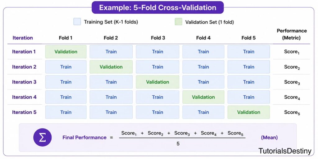
The model trains on four folds and tests on one.

This process repeats until every fold has served as the testing dataset.

Visualizing K-Fold Validation

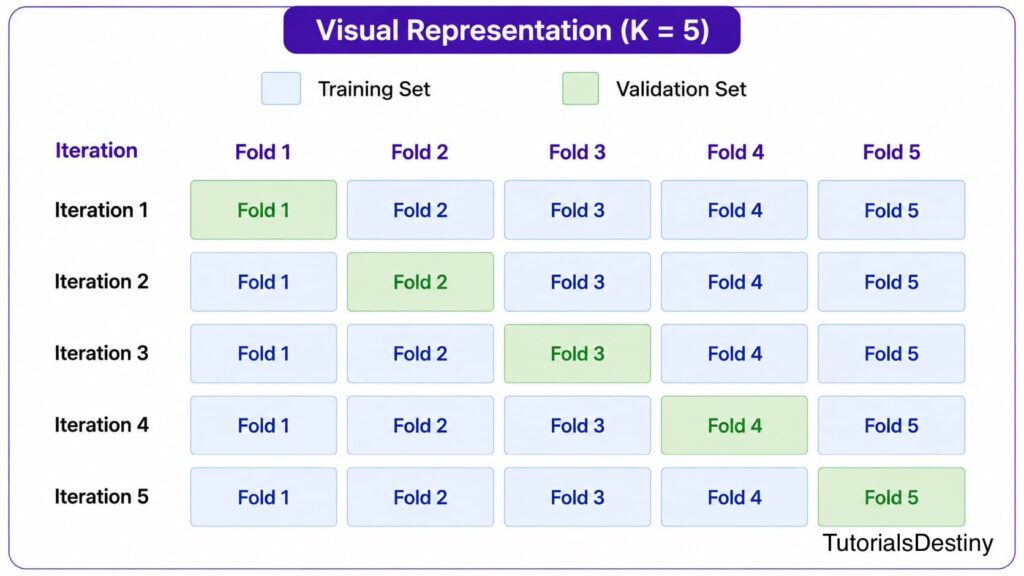
Final performance is calculated as the average across all rounds.

Benefits of Cross-Validation

Cross-validation provides:

• More reliable estimate of model performance compared to a single train-test split.
• Better model comparison.
• Helps detect overfitting and selection bias.
• Efficient use of data: Every data point is used for both training and validation.

For these reasons, it is widely used in professional Machine Learning workflows.

Common Evaluation Mistakes

Even experienced practitioners can make evaluation errors. Understanding these mistakes helps prevent misleading results.

Mistake 1: Evaluating on Training Data

Testing a model using the same data used for training produces unrealistic performance estimates. The model may simply memorize examples. Always use separate testing data.

Mistake 2: Using Accuracy Alone

As we have seen, accuracy can be highly misleading. Always consider additional metrics.

Mistake 3: Ignoring Class Imbalance

Imbalanced datasets require specialized evaluation approaches. Ignoring imbalance often leads to poor real-world performance.

Mistake 4: Data Leakage

Data leakage occurs when information from testing data unintentionally influences training. This can produce artificially inflated results.

Data leakage is one of the most dangerous evaluation mistakes.

Mistake 5: Small Test Datasets

Tiny testing datasets may produce unstable results. Larger, representative datasets provide more reliable evaluations.

Evaluation in Modern AI Systems

Evaluation becomes even more complex in advanced AI applications. Different domains use specialized metrics.

Evaluation in Computer Vision

Computer Vision systems often use:

• Accuracy
• Precision
• Recall
• Intersection over Union (IoU)
• Mean Average Precision (mAP)

These metrics evaluate object detection and image recognition performance.

Evaluation in Natural Language Processing

NLP systems commonly use:

• Precision
• Recall
• F1 Score
• BLEU Score
• ROUGE Score
• Perplexity

These metrics assess language understanding and text generation quality.

Evaluation in Generative AI

Modern Generative AI systems present unique challenges.

Examples include:

• Chatbots
• Image generators
• Content creation systems

Evaluation may involve:

• Human feedback
• User satisfaction
• Relevance
• Creativity
• Safety

Unlike traditional Machine Learning, evaluation often combines quantitative and qualitative approaches.

Interview Corner

Frequently Asked Interview Questions

Why is accuracy not always a good metric?

Accuracy can be misleading when datasets are imbalanced or when certain errors are more costly than others.

What is the difference between precision and recall?

Precision measures prediction quality.

Recall measures detection capability.

When should F1 Score be used?

When precision and recall are both important, especially for imbalanced datasets.

What is Cross-Validation?

A technique that repeatedly trains and tests models on different subsets of data to produce more reliable evaluation estimates.

Why is ROC-AUC useful?

It evaluates model performance across multiple classification thresholds rather than relying on a single threshold.

Key Takeaways

• Evaluation determines whether a model is suitable for deployment.
• Different tasks require different evaluation metrics.
• Accuracy alone is often insufficient.
• Precision, recall, and F1 Score provide deeper insight.
• ROC-AUC and Precision-Recall Curves evaluate classification performance across thresholds.
• MAE, MSE, RMSE, and R² are essential regression metrics.
• Cross-validation improves evaluation reliability.
• Imbalanced datasets require special consideration.
• Modern AI systems often use specialized evaluation approaches.k

These concepts form the foundation upon which modern Artificial Intelligence systems are built.

What’s Next?

➡ Module 3: Neural Networks and Deep Learning

In the next module, you will explore the technology that powers many of today’s most advanced AI systems, including image recognition platforms, voice assistants, recommendation engines, autonomous systems, and generative AI models.

Next Lesson

➡ Module 3 – Lesson 1: Introduction to Neural Networks

From Biological Neurons to Artificial Intelligence

In this lesson, you will learn:

• How biological neurons inspired artificial neural networks
• The structure of artificial neurons
• Perceptrons and activation functions
• Neural network architecture
• How neural networks learn complex patterns
• Why deep learning transformed modern AI

[Begin Module 3 →]