Gradient Descent and Optimization Algorithms

Understanding the Need for Optimization

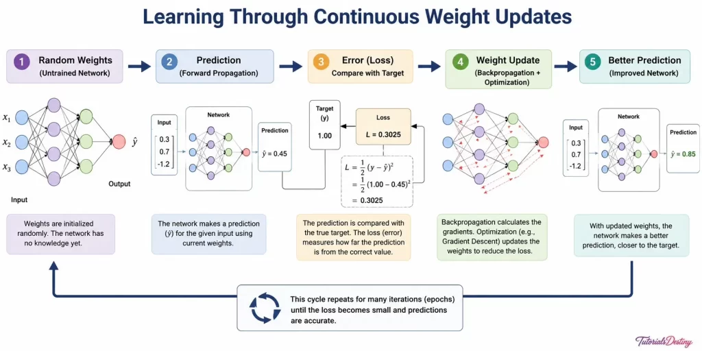
By the end of the previous lesson, our neural network had completed an entire learning cycle. It generated a prediction through forward propagation, measured the prediction error using a loss function, and used backpropagation to calculate how much each weight contributed to that error. At this stage, the network has gained valuable feedback about its performance, but it has not actually learned anything yet.

The gradients calculated during backpropagation indicate which direction each weight should move to reduce the error. However, gradients are only mathematical instructions. They do not modify the network’s parameters automatically. If the training process stopped here, the neural network would simply produce the same predictions every time it encountered similar data, regardless of how accurately the gradients were calculated.

This naturally raises an important question:

How does a neural network use these gradients to improve its predictions?

The answer lies in optimization. Optimization is the process of updating the network’s weights and biases using the information provided by backpropagation. Every improvement made by a neural network—whether it is identifying an object more accurately, translating a sentence more naturally, or recognizing a spoken word more precisely—is the result of optimization.

Why Weight Updates Are Essential

Every neural network begins its journey with randomly initialized weights. Because these values are chosen before the model has seen any training data, the network has no understanding of the patterns it is expected to learn. Its first predictions are therefore often inaccurate.

Consider a neural network trained to classify different types of fruits. During its initial training iterations, it may incorrectly identify an apple as a tomato or confuse an orange with a grapefruit. These mistakes are expected because the network has not yet learned the visual characteristics that distinguish one fruit from another.

After each incorrect prediction, the network measures the error and calculates the gradients. However, these calculations become meaningful only when the weights are updated. Each update is usually very small, but it moves the model slightly closer to the correct solution. Over thousands of training iterations, these tiny improvements accumulate, allowing the network to recognize increasingly complex patterns with remarkable accuracy.

From Optimization to Gradient Descent

Optimization gives a neural network a way to turn the feedback produced by backpropagation into actual learning. The gradients calculated during backpropagation tell us how the loss changes with respect to each weight and bias, but the gradients themselves do not change the network’s parameters. The optimizer must use this information to determine how those parameters should be adjusted.

The fundamental objective is straightforward: find parameter values that reduce the loss and improve the network’s predictions. Rather than searching for better weights randomly or making large unpredictable changes, optimization algorithms make a sequence of controlled updates. Each update moves the parameters toward a region where the network produces a lower prediction error.

One of the most fundamental algorithms for achieving this is Gradient Descent. It uses the gradients calculated during backpropagation to determine the direction in which the parameters should move. The gradient indicates how the loss changes as a parameter changes, while the learning rate controls the size of the adjustment.

After each update, the network processes more training data, calculates the loss again, computes new gradients, and updates its parameters once more. This cycle continues throughout training. A single update may have only a small effect, but thousands of carefully calculated updates can gradually transform a randomly initialized network into a model capable of recognizing complex patterns and making accurate predictions.

Understanding the Idea Behind Gradient Descent

Imagine standing on a mountain covered in thick fog. Your goal is to reach the lowest point in the valley, but you cannot see the entire landscape because the fog blocks your view. Instead of searching randomly, you observe the slope beneath your feet and take a small step in the direction that leads downward.

After taking that step, you stop, observe the slope again, and repeat the process. Every new step brings you a little closer to the valley. Although you never see the complete mountain, continuously following the downward slope eventually guides you to a much lower point.

Gradient Descent works in exactly the same way. Instead of moving across a mountain, it moves through a mathematical surface called the loss landscape. The objective is not to reduce altitude but to reduce the prediction error. During every training iteration, the algorithm examines the gradients, identifies the direction in which the loss decreases, and updates the network’s weights accordingly. These updates are intentionally small, allowing the model to improve steadily without making unstable jumps.

Why Is It Called Gradient Descent?

The name Gradient Descent is derived from two important concepts.

The gradient represents the slope of the loss function. It tells the optimizer how the loss changes when a particular weight is increased or decreased. A large gradient indicates that the loss is highly sensitive to that parameter, while the sign of the gradient determines the direction in which the parameter should be adjusted, while a small gradient suggests that the weight is already close to a good value.

The word descent refers to the process of moving downhill toward a lower loss. Instead of climbing toward higher error values, the optimizer always attempts to move in the direction that reduces the loss as much as possible.

Together, these two ideas describe the complete purpose of the algorithm: use the slope of the loss function to move toward lower prediction error.

The Learning Cycle Continues

At this stage, we have connected the two most important parts of neural network training. Backpropagation calculates the gradients, while Gradient Descent uses those gradients to update the network’s parameters. These two algorithms work together throughout the training process, repeating the same cycle until the model reaches an acceptable level of accuracy.

The next question is naturally how these weight updates are actually calculated. To answer that, we need to understand the mathematical rule that Gradient Descent follows every time it adjusts a neural network’s parameters.

How Gradient Descent Updates the Weights

Understanding the idea behind Gradient Descent is only the first step. To appreciate how a neural network actually learns, we need to examine how the algorithm updates its weights after every training iteration.

As we learned in the previous lesson, backpropagation calculates the gradient for every trainable parameter in the network.

Gradient Descent uses these gradients to determine the next value of every weight. Instead of making large changes, it performs a series of small and controlled updates. This gradual approach allows the network to improve steadily while maintaining stable learning.

The Weight Update Rule

The mathematical rule followed by Gradient Descent is surprisingly simple. After calculating the gradient, the algorithm updates each weight using the following equation:

Although the equation may appear intimidating at first, every symbol has a clear meaning.

$w_{\text{new}} = w_{\text{old}} – \eta \frac{\partial L}{\partial w}$

Where:

$w_{new}$ represents the updated weight.
$w_{old}$ is the current weight before the update.
$\eta (eta)$ is the learning rate, which controls the size of the update.
$\frac{\partial L}{\partial w}$ is the gradient of the loss function with respect to the weight.

The equation simply tells the optimizer to subtract a small portion of the gradient from the current weight. By doing this repeatedly, the network gradually moves toward a set of weights that produces lower prediction error.

Understanding the Formula Intuitively

Rather than memorizing the equation, it is more useful to understand what it is trying to achieve.

Imagine that you are adjusting the focus of a camera. If the image appears blurry, you do not rotate the focus ring as far as possible in a single attempt. Instead, you make a small adjustment, observe whether the image becomes clearer, and continue making fine corrections until the picture is sharp.

Gradient Descent follows the same philosophy.

After every prediction, the optimizer examines the feedback received through the gradients and makes a small correction to each weight. If the correction reduces the prediction error, the network has moved in the right direction. The process is then repeated for the next training example or batch, allowing the model to improve little by little.

This strategy may seem slow, but it is one of the main reasons neural networks learn so reliably.

A Simple Numerical Example

Suppose a neural network has one weight with a current value of 0.80. During backpropagation, the gradient for this weight is calculated as 0.20, and the learning rate is 0.10.

Applying the update rule gives:

Current weight: 0.80
Gradient: 0.20
Learning rate: 0.10
Updated weight: 0.80 − (0.10 × 0.20) = 0.78

Notice that the weight changes only from 0.80 to 0.78. The adjustment is small, but that is exactly the goal. Instead of making dramatic corrections after every mistake, the optimizer gradually refines the network’s knowledge through thousands of controlled updates.

The Importance of Controlled Updates

It may seem tempting to change the weights by a large amount so that the network learns more quickly. In practice, however, this often leads to unstable training.

Imagine trying to park a car in a narrow space. If you turn the steering wheel sharply after every small deviation, the car will keep swinging from one side to the other. Smooth, controlled steering produces a much better result.

The same principle applies to Gradient Descent. Small weight updates help the optimizer move steadily toward lower prediction error without overshooting the optimal solution. Although this requires many iterations, it produces a more stable and reliable learning process.

The size of these updates is controlled by a parameter known as the learning rate. Choosing an appropriate learning rate is one of the most important decisions in deep learning because it determines how quickly or slowly the network learns.

The gradient determines the direction of the update, but another question remains: how large should that update be? This is where the learning rate becomes important.

The Learning Rate: Controlling the Speed of Learning

Gradient Descent updates the weights by making small adjustments after every training iteration. While the direction of these updates is determined by the gradients, another factor decides how large each update should be. This factor is known as the learning rate.

The learning rate is one of the most important hyperparameters in deep learning because it directly influences how quickly a neural network learns. Every time the optimizer updates the weights, the learning rate determines the size of the step taken toward reducing the loss. If this value is chosen carefully, the network learns efficiently and converges toward a good solution. If it is chosen poorly, training can become painfully slow or fail altogether.

For this reason, selecting an appropriate learning rate is often one of the first tasks performed when training a deep learning model.

What Is the Learning Rate?

The learning rate, commonly represented by the Greek letter η (eta), is a numerical value that controls the size of each weight update during optimization.

Think of Gradient Descent as a person walking downhill toward the lowest point of a valley. The gradients indicate which direction to walk, while the learning rate determines how big each step should be.

A larger learning rate means bigger steps, allowing the model to move more quickly across the loss landscape. A smaller learning rate results in shorter, more careful steps, making learning slower but often more stable.

Finding the right balance between these two extremes is essential for successful training.

When the Learning Rate Is Too Small

Suppose a person wants to walk one kilometre but takes steps that are only a few millimetres long. Although they are moving in the correct direction, reaching the destination will take an unnecessarily long time.

The same thing happens when the learning rate is extremely small.

Each weight update becomes so tiny that the network requires an enormous number of training iterations before any noticeable improvement occurs. The loss decreases very slowly, increasing both the training time and computational cost.

Although a small learning rate often produces stable learning, it can make training inefficient, especially for large neural networks containing millions of parameters.

When the Learning Rate Is Too Large

Now imagine the opposite situation. Instead of taking small, careful steps downhill, the person begins making huge leaps. Rather than approaching the valley smoothly, they repeatedly jump over the lowest point, moving from one side of the valley to the other.

An excessively large learning rate causes a neural network to behave in a similar way.

The optimizer makes weight updates that are too large, causing the loss to fluctuate or even increase instead of decreasing. In some cases, the model may never converge because it continuously overshoots the optimal solution.

Instead of learning efficiently, the network becomes unstable and struggles to improve.

Finding the Learning Rate Sweet Spot

An effective learning rate strikes a balance between speed and stability.

It should be large enough to allow the model to make meaningful progress during each training iteration, yet small enough to avoid overshooting the optimal solution. With an appropriate learning rate, the loss decreases steadily, and the network converges smoothly toward better-performing weights.

In practice, finding this balance often requires experimentation. Data scientists frequently begin with a commonly used learning rate and adjust it based on the behaviour of the training process. If the loss decreases too slowly, the learning rate may be increased. If the loss becomes unstable or oscillates, the learning rate is usually reduced.

Although there is no universal value that works for every problem, choosing an appropriate learning rate is one of the most influential decisions in deep learning.

Comparison of Small, Optimal, and Large Learning Rates

Learning Rate in Modern Deep Learning

Modern optimization algorithms have made learning rate selection much easier than it was in the early days of deep learning. Optimizers such as RMSProp and Adam automatically adapt the effective learning rate for different parameters during training, allowing the model to learn more efficiently across different regions of the loss landscape.

Despite these advances, the learning rate remains a critical hyperparameter. Even adaptive optimizers require an initial learning rate, and choosing an unsuitable value can still lead to slow learning or unstable training.

This highlights an important principle of deep learning: the optimizer determines how weights are updated, while the learning rate determines how aggressively those updates are applied. Both work together to guide the neural network toward a better solution.

Key Points

The learning rate (η) controls the size of every weight update during optimization.
A very small learning rate results in slow but stable learning.
A very large learning rate can cause unstable training and prevent convergence.
An appropriate learning rate balances training speed with stability.
Modern optimizers such as Adam and RMSProp adapt learning rates automatically, but selecting a suitable initial value is still important.

With the role of the learning rate now established, we are ready to explore the different ways in which Gradient Descent performs weight updates. In the next section, we will compare Batch Gradient Descent, Stochastic Gradient Descent (SGD), and Mini-Batch Gradient Descent, and understand why each approach is suited to different training scenarios.

Types of Gradient Descent

So far, we have learned that Gradient Descent updates a neural network’s weights in order to reduce the prediction error. However, one important question still remains:

How much training data should the algorithm use before updating the weights?

The answer to this question gives rise to three different variants of Gradient Descent. Although all three aim to minimize the loss function, they differ in when they perform weight updates. Some update the weights after processing the entire training dataset, while others update them much more frequently using smaller portions of data.

Understanding these approaches is important because they directly affect training speed, memory usage, convergence, and overall model performance.

Batch Gradient Descent

Batch Gradient Descent processes the entire training dataset before updating the network’s weights.

Suppose a dataset contains 20,000 training examples. Instead of updating the weights after each example, Batch Gradient Descent first performs forward propagation and backpropagation for all 20,000 examples. Once the gradients from the complete dataset have been calculated, it performs a single weight update.

Because the gradients are calculated using the entire dataset, the update direction is highly accurate and stable. However, this approach requires significant computational resources and memory, especially when working with millions of training samples. As datasets continue to grow, waiting for the entire dataset before making a single update becomes increasingly inefficient.

Advantages

Produces stable and consistent gradient estimates.
Less affected by random fluctuations during training.
Suitable for relatively small datasets.

Limitations

Slow training on large datasets.
Requires high memory usage.
Performs only one weight update per training epoch.

Stochastic Gradient Descent (SGD)

To overcome the limitations of Batch Gradient Descent, researchers introduced Stochastic Gradient Descent (SGD).

Instead of waiting for the complete dataset, SGD updates the weights after processing a single training example. Each prediction is immediately followed by loss calculation, backpropagation, and a weight update.

This frequent updating allows the model to start learning much earlier. Since every training example slightly changes the weights, SGD often reaches useful solutions much faster than Batch Gradient Descent.

However, because each update is based on only one example, the gradients are noisy. As a result, the optimization path often appears irregular, and the loss may fluctuate before eventually converging.

Advantages

Faster learning.
Requires less memory.
Can escape shallow local minima due to its noisy updates.

Limitations

Training path is less stable.
Loss values fluctuate significantly.
May require more iterations before convergence.

Mini-Batch Gradient Descent

Modern deep learning combines the strengths of both previous approaches through Mini-Batch Gradient Descent.

Instead of processing the entire dataset or a single example, the training data is divided into small batches, commonly containing 32, 64, 128, or 256 training examples. After processing one mini-batch, the optimizer updates the network’s weights before moving to the next batch.

This approach achieves an excellent balance between computational efficiency and stable learning. The gradients are more reliable than those of SGD because they are calculated from multiple examples, while the updates are much more frequent than those of Batch Gradient Descent.

For this reason, Mini-Batch Gradient Descent has become the standard training strategy for most modern deep learning frameworks, including TensorFlow and PyTorch.

Advantages

Faster than Batch Gradient Descent.
More stable than SGD.
Efficient use of modern CPUs and GPUs.
Suitable for large datasets.

Limitations

Batch size must be selected carefully.
Very small or very large batches can reduce training efficiency.

Comparing the Three Approaches

Although all three algorithms follow the same principle of reducing the loss, they differ in how frequently they update the network’s weights.

Feature	Batch GD	Stochastic GD	Mini-Batch GD
Training data used per update	Entire dataset	One training example	Small batch of examples
Weight updates	Once per epoch	After every example	After every mini-batch
Training speed	Slow	Fast	Fast and efficient
Memory requirement	High	Low	Moderate
Stability	High	Low	High
Common use today	Rare	Limited	Most widely used

Mini-Batch Gradient Descent offers the best balance between speed, stability, and computational efficiency, making it the preferred choice for training most modern deep learning models.

BGD is precise but slow. SGD is fast but noisy. Mini-batch gives the best trade-off and is the most commonly used approach in deep learning.

Why Modern Deep Learning Prefers Mini-Batches

Today’s neural networks are trained on enormous datasets containing millions of images, documents, audio recordings, and videos. Processing an entire dataset before every weight update would be impractical, while updating the weights after every single example would introduce excessive randomness.

Mini-Batch Gradient Descent provides an effective compromise. It allows GPUs to process data efficiently through parallel computation while maintaining stable gradient estimates. This combination of speed, accuracy, and scalability explains why almost every modern deep learning application—from image recognition and speech processing to large language models—uses mini-batch training.

Mini-batches make gradient-based training efficient, but the basic update can still be improved. This leads to advanced optimization algorithms such as Momentum, RMSProp, and Adam.

Advanced Optimization Algorithms

Mini-Batch Gradient Descent has become the standard approach for training modern neural networks because it offers an excellent balance between speed and stability. However, even Mini-Batch Gradient Descent is not without limitations. As neural networks became deeper and datasets grew larger, researchers discovered that the basic Gradient Descent algorithm often learned more slowly than desired and sometimes struggled to reach the best solution.

To address these challenges, several advanced optimization algorithms were developed. Rather than replacing Gradient Descent, these optimizers build upon its core principle while introducing new strategies that make training faster, smoother, and more efficient.

Among the many optimizers proposed over the years, four have become especially important: Stochastic Gradient Descent (SGD), Momentum, RMSProp, and Adam.

Stochastic Gradient Descent (SGD)

Although we discussed Stochastic Gradient Descent as one of the variants of Gradient Descent, it is also widely used as an optimizer in deep learning. In practice, when people refer to the SGD optimizer, they usually mean Mini-Batch Gradient Descent with optional improvements such as momentum.

The SGD optimizer updates the network’s weights after processing each mini-batch. These frequent updates allow the model to begin learning immediately instead of waiting for an entire training epoch to finish. As a result, SGD is computationally efficient and works well for many machine learning problems.

However, the optimizer follows only the current gradient while deciding the next update. It has no memory of previous steps. This can cause the optimization path to fluctuate, especially when the loss landscape contains steep valleys or irregular surfaces.

Advantages

Simple and easy to implement.
Requires relatively little memory.
Performs well on many machine learning tasks.

Limitations

Training can be noisy.
May converge slowly.
Often oscillates while approaching the minimum.

Momentum Optimizer

Imagine pushing a heavy ball down a hill. The ball does not stop after every small movement. Instead, it builds momentum and continues rolling in the same direction.

The Momentum Optimizer applies this same idea to neural network training.

Instead of relying only on the current gradient, Momentum also considers the direction of previous updates. If several consecutive updates point in the same direction, the optimizer gradually increases its movement in that direction. This helps the network move more quickly through flat regions while reducing the side-to-side oscillations that often occur during optimization.

As a result, Momentum usually converges faster than standard SGD and follows a much smoother path toward the minimum.

RMSProp Optimizer

Not every weight in a neural network learns at the same speed. Some parameters require large adjustments, while others need only small corrections. Using the same learning rate for every weight can therefore slow down the training process.

RMSProp (Root Mean Square Propagation) solves this problem by adapting the learning rate for each parameter individually. Weights that receive consistently large gradients automatically take smaller steps, while weights with smaller gradients are allowed to take relatively larger steps.

This adaptive behaviour enables the optimizer to learn more efficiently, especially when the loss landscape contains regions with very different gradient magnitudes. RMSProp became particularly popular for training Recurrent Neural Networks (RNNs) because it improves stability during long training sequences.

Adam Optimizer

Among all optimization algorithms, Adam (Adaptive Moment Estimation) is the most widely used in modern deep learning.

Adam combines the strengths of Momentum and RMSProp into a single optimization algorithm. Like Momentum, it remembers the direction of previous updates, allowing it to move smoothly toward the minimum. Like RMSProp, it automatically adjusts the learning rate for each parameter, enabling different parts of the network to learn at different speeds.

Because of this combination, Adam generally converges faster, requires less manual tuning, and performs well across a wide variety of deep learning tasks. Whether the application involves image classification, natural language processing, speech recognition, or large language models, Adam is often the optimizer chosen as the default starting point.

Comparing Popular Optimizers

Although all optimizers aim to minimize the loss function, they use different strategies to update the network’s weights.

Optimizer	Key Idea	Strength	Limitation
SGD	Uses the current gradient	Simple and memory efficient	Can converge slowly
Momentum	Uses previous updates to accelerate learning	Faster and smoother convergence	Requires tuning of momentum parameter
RMSProp	Adapts learning rate for each parameter	Stable training for deep networks	Additional computations required
Adam	Combines Momentum and RMSProp	Fast, adaptive, and widely applicable	May not always produce the best generalization for every problem

For most practical deep learning applications, Adam is considered the default optimizer because it offers an excellent balance between speed, stability, and ease of use. Nevertheless, experienced practitioners often experiment with different optimizers to achieve the best performance for a specific task.

Optimization in Practice

Every modern deep learning framework—including TensorFlow, PyTorch, and Keras—provides built-in implementations of these optimizers. In many projects, changing the optimizer requires modifying only a single line of code, yet this small change can have a significant impact on training speed and model performance.

Choosing the right optimizer is therefore an important part of building an effective neural network. While Gradient Descent provides the foundation for learning, advanced optimizers refine that process, allowing today’s AI systems to train efficiently on datasets containing millions—or even billions—of examples.

With this understanding of optimization algorithms, we have now completed the journey from calculating gradients to using them to improve a neural network. In the final part of this lesson, we will summarize the key concepts, review the main takeaways, and reinforce your understanding through practice questions.

Lesson Summary

In this lesson, we explored how a neural network transforms the feedback generated during backpropagation into meaningful learning through optimization. We began by understanding why optimization is necessary and learned that calculating gradients alone is not enough. A neural network improves only when those gradients are used to update its weights and biases after every training iteration.

We then introduced Gradient Descent, the fundamental optimization algorithm that forms the basis of modern deep learning. Rather than making random adjustments, Gradient Descent uses the gradients calculated during backpropagation to move the network’s parameters in the direction that reduces the prediction error. Although each update is small, thousands of such updates gradually transform a randomly initialized network into a model capable of making highly accurate predictions.

Another important concept discussed in this lesson was the learning rate. We saw how this single hyperparameter controls the size of every weight update and directly influences the speed and stability of learning. A learning rate that is too small slows the training process, while one that is too large can prevent the model from converging to a good solution. Selecting an appropriate learning rate is therefore an essential part of training any deep neural network.

We also compared the three major variants of Gradient Descent—Batch Gradient Descent, Stochastic Gradient Descent, and Mini-Batch Gradient Descent. Although each follows the same objective of minimizing the loss function, they differ in how frequently they update the network’s weights. Among these approaches, Mini-Batch Gradient Descent has become the preferred choice for most modern deep learning applications because it provides an excellent balance between computational efficiency and stable learning.

Finally, we explored the evolution of optimization algorithms beyond basic Gradient Descent. Optimizers such as Momentum, RMSProp, and Adam build upon the same core principle while introducing strategies that improve convergence speed, reduce oscillations, and adapt the learning process. These optimizers have become indispensable tools for training today’s deep learning models efficiently.

By the end of this lesson, we have completed an important milestone in our understanding of neural networks. We now know how a network generates predictions, measures its errors, computes gradients, and updates its parameters to learn from experience. Together, these concepts form the foundation of the training process used by virtually every modern deep learning system.

Key Takeaways

After completing this lesson, you should be able to:

Explain why optimization is essential in neural network training.
Describe how Gradient Descent updates network weights.
Interpret the Gradient Descent weight update rule.
Explain the role of the learning rate during optimization.
Compare Batch, Stochastic, and Mini-Batch Gradient Descent.
Distinguish between the SGD, Momentum, RMSProp, and Adam optimizers.
Explain why Mini-Batch Gradient Descent and Adam are widely used in modern deep learning.

Practice Questions

Conceptual Questions

Why is optimization necessary after backpropagation?
Explain the working principle of Gradient Descent.
What information do gradients provide during optimization?
How does the learning rate influence the training process?
What happens if the learning rate is too small or too large?
Compare Batch Gradient Descent, Stochastic Gradient Descent, and Mini-Batch Gradient Descent.
Why is Mini-Batch Gradient Descent preferred in modern deep learning?
How does the Momentum optimizer improve standard Gradient Descent?
What problem does RMSProp solve?
Why is Adam considered the default optimizer for many deep learning applications?

Looking Ahead

Although optimization enables a neural network to learn by updating its weights, successful training involves more than choosing the right optimizer. Deep neural networks often face practical challenges such as unstable gradients, overfitting, poor weight initialization, and slow convergence. If these challenges are not addressed, even the most advanced optimization algorithms may struggle to produce good results.

In the next lesson, Training Challenges and Best Practices, we will explore the common obstacles encountered while training deep neural networks and study the techniques used to overcome them. You will learn about vanishing and exploding gradients, weight initialization methods, batch normalization, dropout, regularization, early stopping, and other best practices that help build stable, accurate, and efficient deep learning models.