Training Deep Neural Networks

How Do Neural Networks Learn?

In the previous lessons, we explored how neurons are organized into layers and how different architectures enable deep learning models to solve complex problems. We discovered that hidden layers progressively transform raw input into meaningful representations, allowing a network to recognize images, understand language, and make intelligent predictions.

However, one fundamental question still remains unanswered:

How does a neural network actually become intelligent?

When a neural network is created, it does not possess any knowledge. It cannot distinguish a cat from a dog, predict house prices, translate languages, or detect fraudulent transactions. At the beginning, all of its connection weights are initialized with small random values. Consequently, its predictions are little better than random guesses.

Learning occurs only after the network is exposed to data repeatedly. During training, the network compares its predictions with the correct answers, measures how far its predictions are from reality, identifies which connections contributed to the error, and adjusts those connections to improve future predictions.

This continuous cycle of prediction → error measurement → correction → improvement lies at the heart of every deep learning model.

Rather than memorizing answers, the network gradually discovers patterns hidden within the data by making thousands or even millions of tiny adjustments to its internal parameters.

Understanding this learning process is essential because nearly every modern deep learning algorithm—whether it powers ChatGPT, self-driving cars, medical diagnosis systems, or recommendation engines—relies on the same fundamental training principles.

Why Training Is Necessary

Imagine asking a student to solve a difficult mathematics problem without ever teaching them the underlying concepts. The student’s first attempt is likely to be incorrect. After reviewing the mistakes and receiving feedback, the student learns what went wrong and performs better on the next attempt.

A neural network learns in a remarkably similar way.

It begins by making a prediction based on its current knowledge. The prediction is then compared with the correct answer, and the difference between the two is calculated as an error. This error serves as feedback, guiding the network on how its internal parameters should change.

Over many training iterations, the network gradually reduces its errors and becomes increasingly accurate. This process is known as training.

Unlike traditional programming, where developers explicitly write rules, deep learning allows the network to discover these rules automatically from examples.

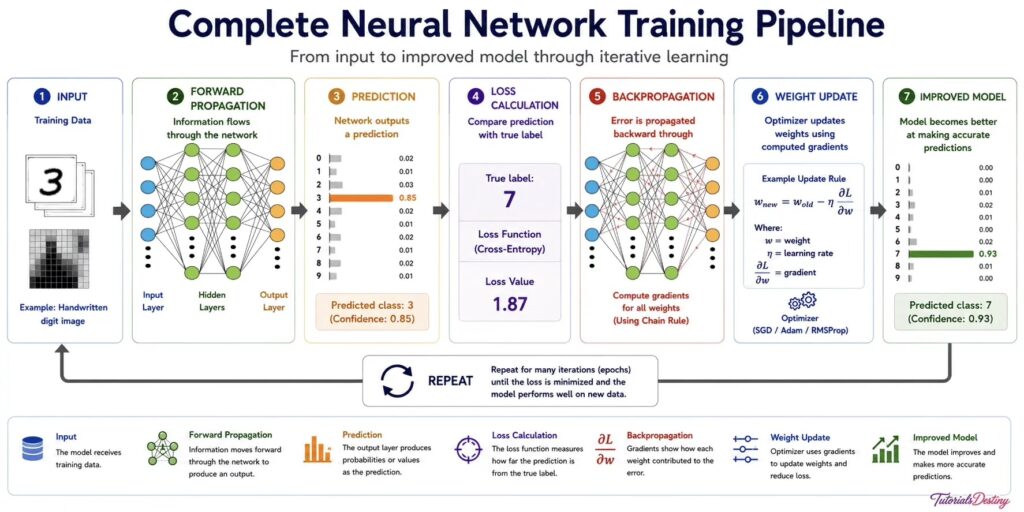
The Complete Learning Cycle

Every deep neural network follows the same fundamental learning cycle, regardless of its architecture.

The training data is provided to the network.
The network performs forward propagation to generate a prediction.
A loss function measures the prediction error.
Backpropagation calculates how much each weight contributed to the error.
An optimizer updates the weights to reduce future errors.
The process repeats for many epochs until the model converges.

Although each of these steps involves sophisticated mathematics, the overall workflow is surprisingly intuitive: predict, measure, learn, and improve.

An Everyday Example

Consider a neural network designed to classify handwritten digits. Suppose the input image contains the digit 3.

During its first training iteration, the network predicts:

Prediction: 8

Actual Label: 3

Clearly, the prediction is incorrect.

The loss function calculates how far the prediction is from the correct answer. Backpropagation then identifies which neurons and weights contributed most to the mistake. Finally, the optimizer adjusts those weights slightly.

When the same or similar images are presented again, the network is more likely to predict the correct digit.

After thousands of iterations, the model becomes highly accurate—not because it memorized every image, but because it learned the underlying visual patterns that distinguish one digit from another.

Learning Through Small Improvements

One common misconception is that neural networks make large corrections after each mistake.

In reality, learning happens through many small adjustments.

Every training step modifies the network’s weights only slightly. These tiny improvements accumulate over time, gradually steering the model toward better performance.

This incremental learning process offers several advantages:

It allows the network to learn stable and generalized patterns.
It reduces the risk of drastic parameter changes that could destabilize training.
It enables the model to adapt to increasingly complex relationships within the data.

The idea of improving through countless small updates is one of the key reasons deep learning models can achieve remarkable performance on challenging tasks.

Key Components of Neural Network Training

Although the training process appears seamless, it is built upon several interconnected components.

Throughout this lesson, we will explore each of these in detail:

Forward Propagation – Producing predictions from input data.
Loss Function – Measuring prediction error.
Backpropagation – Calculating gradients and identifying how weights should change.

Together, these concepts explain how a neural network makes predictions, measures its mistakes, and learns where improvements are needed. They provide the conceptual foundation upon which the optimization techniques explored in the next lesson are built.

Forward Propagation: From Input Data to Prediction

A neural network improves by repeatedly making predictions, measuring its errors, and adjusting its internal parameters. However, before the network can learn from its mistakes, it must first produce a prediction.

The process of generating this prediction is known as forward propagation.

Every neural network, whether it is a simple Feedforward Neural Network, a Convolutional Neural Network, or a Transformer, begins its computation with a forward pass. It is the first stage of the learning process and serves as the foundation upon which backpropagation and optimization are built.

In this section, we will explore how information travels through a neural network, how each neuron processes incoming data, and how these computations ultimately produce a prediction.

What is Forward Propagation?

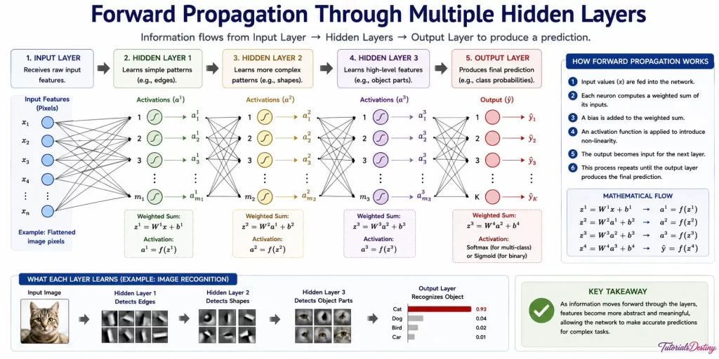
Forward propagation is the process by which input data flows through a neural network to produce an output prediction.

Information always moves in one direction:

Input Layer → Hidden Layer(s) → Output Layer

At each neuron, the received inputs are combined using learned weights and a bias. The result is then passed through an activation function before being forwarded to the next layer.

This process continues until the output layer generates the network’s final prediction.

Unlike backpropagation, which updates the network’s parameters, forward propagation performs only one task: computing predictions using the current values of the weights and biases.

Why Forward Propagation Is Important

Every learning cycle begins with a prediction.

Without forward propagation:

The network cannot generate an output.
The prediction error cannot be calculated.
Backpropagation cannot determine how the weights should change.
The optimizer has no information to improve the model.

In other words, every subsequent step in neural network training depends on the successful completion of forward propagation.

Think of it as the first step in a student’s learning process. Before a teacher can correct an answer, the student must first attempt the question.

Similarly, the neural network must first predict before it can learn.

The Journey of Information

Imagine a neural network trained to classify handwritten digits.

An image of the digit 3 is presented to the network.

The learning process begins with the input layer, where each neuron receives one numerical value representing a pixel intensity from the image.

These values are then passed to the first hidden layer.

Each hidden neuron performs three operations:

Receives all input values.
Multiplies each input by its corresponding weight.
Adds a bias term.

The neuron then applies an activation function to determine its output. This output becomes the input for the next hidden layer.

The same sequence repeats until information reaches the output layer, where the network produces probabilities for each possible digit.

Finally, the digit with the highest probability becomes the model’s prediction.

The Three Operations Inside Every Neuron

Although modern neural networks may contain millions of neurons, every neuron performs the same three fundamental operations.

Step 1: Weighted Sum

Each input is multiplied by its corresponding weight.

Features considered more important receive larger weights, while less relevant features receive smaller weights.

The neuron then adds all weighted inputs together.

For example,

Input 1 × Weight 1
Input 2 × Weight 2
Input 3 × Weight 3

All these values are summed to produce the neuron’s preliminary output.

This weighted sum determines how strongly the neuron should respond to the incoming information.

Step 2: Adding the Bias

The weighted sum alone is often insufficient. A bias is added before applying the activation function.

The bias acts as an adjustable offset that allows the neuron to shift its decision boundary.

Without bias, neurons would have limited flexibility and many useful patterns could not be learned effectively.

One can think of the bias as a starting point that helps the neuron decide when it should become active.

Step 3: Activation Function

The weighted sum and bias are then passed through an activation function. The activation function introduces non-linearity, allowing neural networks to solve complex problems beyond simple linear relationships.

Depending on the chosen activation function, the neuron may:

Pass the value almost unchanged.
Compress it into a probability.
Ignore negative values.
Restrict it within a fixed range.

Without activation functions, stacking multiple neural layers would be equivalent to using a single linear model, eliminating most of the power of deep learning.

Forward Propagation Across Multiple Layers

Forward propagation is not performed only once. Instead, the process repeats at every hidden layer.

Each layer receives the outputs from the previous layer, performs its own computations, and generates a new set of features.

As information progresses through the network, these features become increasingly abstract.

For example:

Layer 1 may identify edges.

Layer 2 combines edges into simple shapes.

Layer 3 recognizes meaningful object parts.

Layer 4 identifies complete objects.

The output layer finally converts these learned representations into a prediction.

This gradual refinement of information explains why deep neural networks are capable of recognizing highly complex patterns.

A Simple Numerical Example

Consider a neuron receiving two inputs.

Input 1 = 2
Input 2 = 3

The learned parameters are:

Weight 1 = 0.4
Weight 2 = 0.6
Bias = 0.5

The neuron first computes the weighted sum:

$(2 \times 0.4) + (3 \times 0.6) = 2.6$

Adding the bias gives:

$2.6 + 0.5 = 3.1$

This value is then passed through an activation function.

If the activation function is ReLU, the output remains 3.1, since ReLU keeps all positive values unchanged.

This output is then forwarded to the next layer, where the same process repeats.

Although this example involves only one neuron, a real deep neural network performs millions—or even billions—of such calculations during every forward pass.

Forward Propagation Algorithm

The complete forward propagation process can be summarized as follows:

Receive the input data.
Pass the inputs to the first hidden layer.
Compute the weighted sum for each neuron.
Add the bias.
Apply the activation function.
Forward the outputs to the next layer.
Repeat until the output layer is reached.
Produce the final prediction.

Every prediction generated by a neural network follows this sequence, regardless of the complexity of the architecture.

Applications of Forward Propagation

Forward propagation is the prediction engine behind countless AI systems.

Some examples include:

Face Recognition: Predicting the identity of a person from an image.
Medical Diagnosis: Identifying diseases from X-ray or MRI scans.
Speech Recognition: Converting spoken words into text.
Language Translation: Predicting translated sentences in another language.
Fraud Detection: Determining whether a financial transaction is legitimate or fraudulent.
Recommendation Systems: Suggesting movies, products, or music based on user preferences.

Although these applications differ significantly, they all rely on forward propagation to generate predictions before learning from their errors.

Bridging to the Next Concept

Forward propagation enables the network to produce predictions, but those predictions are rarely perfect during the early stages of training.

This raises another important question:

How does the neural network measure the quality of its predictions?

To improve, the network needs a way to quantify how far its prediction is from the correct answer.

The answer lies in the loss function, which transforms prediction errors into a numerical value that guides the learning process.

Let us explore how loss functions work, why they are essential for neural network training, and how they provide the feedback required for backpropagation and optimization.

Loss Functions: Measuring Prediction Errors

We have already seen how a neural network performs forward propagation to generate predictions. Whether the task is classifying images, translating languages, or predicting house prices, the network always begins by producing an output based on its current knowledge.

However, making a prediction is only the first step.

To learn effectively, the network must determine how accurate its prediction is. It needs a mechanism to compare its prediction with the actual answer and quantify the difference. Without this feedback, the network would have no way of knowing whether it is improving or making poorer predictions.

This is where the loss function comes into play.

A loss function acts as the network’s performance evaluator. It measures the discrepancy between the predicted output and the true target value, producing a numerical score that represents the prediction error. This score becomes the foundation for all subsequent learning, guiding the network toward better performance over time.

What Is a Loss Function?

A loss function is a mathematical function that measures how far a neural network’s prediction is from the correct answer.

After every forward pass, the network compares its predicted output with the actual target value.

If the prediction is correct, the loss is very small.
If the prediction is incorrect, the loss becomes large.

The objective of training is simple:

Minimize the loss so that predictions become increasingly accurate.

A neural network continuously adjusts its weights and biases to reduce this loss over successive training iterations.

Why Is a Loss Function Necessary?

Imagine a student taking an examination.

If the student submits an answer sheet but never receives the results, they have no idea whether their answers were correct or incorrect. Without feedback, there is no opportunity to improve.

A neural network faces the same challenge.

Forward propagation generates predictions, but the network cannot determine whether those predictions are good unless it receives feedback.

The loss function provides that feedback by answering a simple question:

“How wrong is the prediction?”

This information allows the network to identify mistakes and improve during training.

Prediction vs. Loss

Consider a binary image classification task in which a neural network must determine whether an image contains a cat. Instead of directly predicting “Cat” or “Not Cat,” the network outputs the probability that the image belongs to the Cat class.

The loss function then compares this predicted probability with the actual label and computes a numerical error. The larger the difference between them, the higher the loss.

Example 1: Accurate Prediction

Actual Label: Cat
Predicted Probability: P(Cat) = 0.98

Since the network assigns a very high probability to the correct class, the prediction is highly accurate, and the resulting loss is very small.

Example 2: Inaccurate Prediction

Actual Label: Cat
Predicted Probability: P(Cat) = 0.12

Here, the network assigns a very low probability to the correct class, making the prediction highly inaccurate. Consequently, the loss is much larger, indicating that significant adjustments to the network’s weights are needed.

This numerical loss serves as feedback during training. By repeatedly minimizing the loss, the neural network gradually learns to make more accurate predictions.

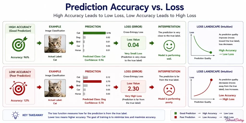
During training, optimization algorithms minimize the loss—not the accuracy directly. As the loss decreases, accuracy often improves as a consequence.

Characteristics of a Good Loss Function

An effective loss function should possess several important properties.

Continuous:The loss should change smoothly as predictions improve or worsen.
Differentiable: The function should be mathematically differentiable so that gradients can be computed during backpropagation.
Sensitive to Errors: Small prediction errors should produce small losses, while larger errors should produce proportionally larger losses.
Easy to Optimize: The loss landscape should guide optimization algorithms efficiently toward better solutions.

Types of Loss Functions

Different machine learning problems require different loss functions. Choosing the appropriate loss function depends primarily on the nature of the prediction task.

Problem Type	Common Loss Function
Linear Regression	Mean Squared Error (MSE)
Binary Classification	Binary Cross-Entropy
Multi-Class Classification	Categorical Cross-Entropy
Object Detection	Combination of Classification and Localization Loss
Image Segmentation	Dice Loss, IoU Loss, Cross-Entropy

Selecting the correct loss function is essential because it directly influences how the model learns.

Mean Squared Error (MSE)

For regression problems, one of the most widely used loss functions is Mean Squared Error (MSE).

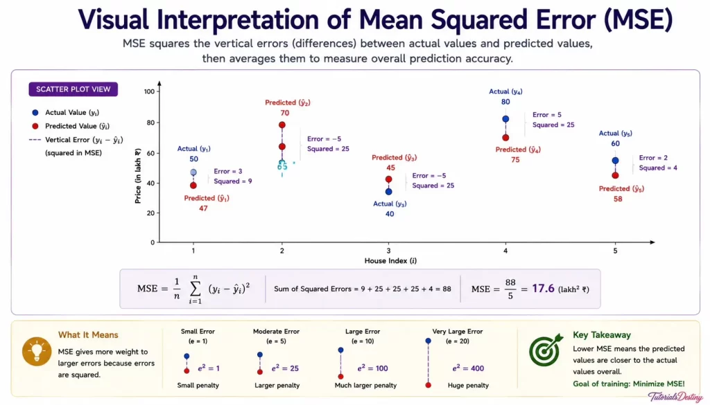
MSE calculates the average squared difference between the predicted values and the actual values.

Where:

$y_i$ $= Actual value$
$\hat{y}_i = Predicted value$
$n = Number of observations$

Squaring the errors ensures that:

Larger mistakes receive greater penalties.
Positive and negative errors do not cancel each other.

Example

Suppose a house actually costs ₹50 lakh, but the model predicts ₹47 lakh.

Prediction Error: ₹3 lakh

Squared Error: (₹3 lakh)²=9

The larger the prediction error, the larger the contribution to the overall loss.

Binary Cross-Entropy Loss

When solving binary classification problems, predicting continuous values is not sufficient. Instead, the network predicts probabilities.

For example:

p(Cat) : 0.95
p(Dog) : 0.05

or

P(Spam) : 0.87
p(Not Spam) : 0.13

In these situations, Binary Cross-Entropy (BCE) is commonly used.

Binary Cross-Entropy heavily penalizes predictions that are both incorrect and made with high confidence.

As a result, the network learns to produce more reliable probability estimates over time.

Categorical Cross-Entropy

Many real-world AI problems involve more than two classes.

For example, a neural network may classify an image into one of several categories:

Cat
Dog
Horse
Bird
Car

In these situations, Categorical Cross-Entropy measures how well the predicted probability distribution matches the correct class.

A correct prediction with high confidence results in a low loss, whereas assigning a high probability to the wrong class produces a much larger loss.

This loss function is widely used in image classification, natural language processing, speech recognition, and many other deep learning applications.

Understanding the Loss Curve

One of the easiest ways to evaluate training progress is by observing the loss curve.

At the beginning of training:

Predictions are mostly incorrect.
Loss is high.

As training continues:

Predictions improve.
Loss decreases.

Eventually:

The model converges.
Loss stabilizes near a minimum value.

A steadily decreasing loss curve indicates that the network is learning effectively.

Suggested Wide Diagram: Training Loss Curve Across Epochs

Loss vs. Accuracy

Many beginners assume that loss and accuracy represent the same thing, but they measure different aspects of model performance.

Accuracy	Loss
Percentage of correct predictions	Numerical measure of prediction error
Easier to interpret	Provides detailed feedback for learning
Used for evaluation	Used during optimization
Higher is better	Lower is better

A model may achieve high accuracy while still having a relatively high loss if it makes a few incorrect predictions with excessive confidence. Therefore, both metrics should be monitored during training.

Applications of Loss Functions

Loss functions are used in virtually every deep learning application.

Healthcare: Measure diagnostic prediction errors.

Autonomous Vehicles: Evaluate mistakes in object detection and lane recognition.

Recommendation Systems: Assess how accurately products or movies are recommended.

Language Models: Measure the quality of predicted words during text generation.

Financial Forecasting: Calculate prediction errors in stock prices and market trends.

Regardless of the application, every deep learning model relies on a suitable loss function to guide learning.

Key Takeaways

A loss function measures how far predictions deviate from the correct answers.
Lower loss indicates better model performance.
Different tasks require different loss functions.
MSE is commonly used for regression problems.
Binary and Categorical Cross-Entropy are widely used for classification.
The loss function provides the feedback required for backpropagation.
Minimizing loss is the primary objective of neural network training.

Backpropagation: How Neural Networks Learn from Their Mistakes

In the previous part of this lesson, we explored the role of the loss function in measuring prediction errors. After every forward pass, the network compares its prediction with the actual target value and computes a numerical loss. This value tells us how wrong the prediction is.

However, knowing that a prediction is wrong is only half of the learning process.

A much more important question now arises:

Which weights caused the error, and how should they be adjusted to improve the next prediction?

Imagine a student receiving only the final exam score without knowing which questions were answered incorrectly. Although the student knows the overall performance, they have no idea which topics require improvement.

A neural network faces the same challenge.

The loss function provides an overall error, but it does not identify which individual connections contributed to that error. The network therefore requires a systematic way to trace the error back through every layer and determine how each weight should change.

This remarkable learning mechanism is called backpropagation.

What Is Backpropagation?

Backpropagation is the algorithm that enables a neural network to learn by calculating how much each weight and bias contributed to the prediction error.

Unlike forward propagation, where information flows from the input layer to the output layer, backpropagation works in the opposite direction.

The error starts at the output layer and travels backward through each hidden layer, allowing every neuron to understand its contribution to the final mistake.

Using this information, the network computes gradients for every trainable parameter. These gradients are then used by an optimizer to update the weights and reduce future errors.

Forward propagation makes predictions, while backpropagation teaches the network how to improve those predictions.

Why Is Backpropagation Necessary?

Consider a deep neural network containing millions of weights.

If the network predicts that an image of a cat is actually a dog, the model clearly needs to improve.

But which of those millions of weights should change?

Should they all increase?

Should they all decrease?

Should some remain unchanged?

Without a systematic learning algorithm, answering these questions would be practically impossible.

Backpropagation solves this problem by calculating the influence of every weight on the final loss.

Instead of randomly modifying parameters, the network makes informed adjustments based on mathematical evidence.

Understanding the Learning Process

Imagine throwing a basketball toward a hoop. If the ball falls short, your brain automatically recognizes the mistake and slightly increases the force on the next attempt. If the ball travels too far, you reduce the force.

Over multiple attempts, your shots become increasingly accurate.

A neural network learns in exactly the same way. Each prediction acts like a practice attempt.

Each loss value provides feedback. Each weight update is a small correction. Over thousands of iterations, these tiny corrections accumulate into highly accurate predictions.

The Backpropagation Workflow

The learning cycle now becomes more complete.

The process consists of the following steps:

Input data enters the network.
Forward propagation produces a prediction.
The loss function measures the prediction error.
Backpropagation computes gradients for every weight.
The optimizer updates the weights.
The network becomes slightly more accurate.
The cycle repeats until the loss becomes sufficiently small.

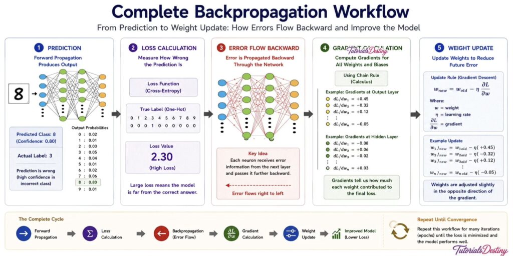
How Error Travels Backward

To understand backpropagation, imagine a simple neural network consisting of:

One input layer
Two hidden layers
One output layer

Suppose the network predicts:

Predicted: Dog

Actual: Cat

The output layer immediately recognizes that the prediction is incorrect because the computed loss is high.

Rather than stopping there, the error begins moving backward through the network.

The output layer first determines how much each of its incoming weights contributed to the mistake.

Next, the second hidden layer receives this information and calculates how much each of its neurons influenced the output layer.

The same process continues backward through every hidden layer until the input layer is reached.

By the end of this backward pass, every weight in the network has received feedback describing how it should change.

This backward flow of error gives the algorithm its name: backpropagation.

Gradients: The Direction of Improvement

The most important quantity computed during backpropagation is the gradient.

A gradient tells the optimizer:

Which direction the weight should move.
How large the adjustment should be.

Think of a hiker standing on a mountain.

The objective is to reach the lowest point in the valley.

The gradient tells the hiker:

Which direction is downhill.
How steep the slope is.

Similarly, gradients guide the optimizer toward lower loss values.

Without gradients, learning would become nothing more than random guessing.

The Chain Rule: Connecting Every Layer

One reason backpropagation is so powerful is that it uses a fundamental concept from calculus known as the Chain Rule.

Each neuron depends on the outputs of the previous layer.

Therefore, changing one weight can indirectly affect many later computations.

The Chain Rule allows the network to calculate how a small change in an early-layer weight influences the final loss.

Rather than treating each layer independently, it links the entire network together into one continuous computational graph.

Although the mathematics behind the Chain Rule can become complex, the underlying intuition is straightforward:

Every layer contributes to the final prediction, so every layer must share responsibility for the final error.

A Simple Numerical Example

Suppose a neuron predicts:

Prediction = 0.80

The actual target is:

Target = 1.00

The prediction error is:

Error = 0.20

Backpropagation determines how much each weight contributed to this error.

For example:

Weight	Gradient
W₁	-0.08
W₂	0.15
W₃	-0.03

These gradients indicate how each weight should be adjusted during the optimization step.

Notice that different weights receive different corrections because they do not all contribute equally to the prediction error.

Why Small Weight Updates Matter

Backpropagation does not dramatically change the network after every mistake.

Instead, it makes small, carefully calculated adjustments.

Large updates could cause the network to overshoot the optimal solution and become unstable.

Small updates allow the model to gradually move toward better predictions while maintaining stable learning.

This is why training often requires thousands of iterations.

Learning is a gradual refinement rather than an instant transformation.

Backpropagation in Deep Networks

Modern neural networks may contain:

Hundreds of layers
Millions of neurons
Billions of trainable parameters

Despite this enormous complexity, backpropagation scales remarkably well because it computes gradients efficiently by reusing intermediate calculations from the forward pass.

Without backpropagation, training today’s large language models, image recognition systems, and speech recognition models would be computationally impractical.

Applications of Backpropagation

Backpropagation is the learning engine behind nearly every deep learning application.

Computer Vision: Improves object recognition by refining convolutional filters.
Natural Language Processing: Updates language model parameters for better text generation and translation.
Speech Recognition: Learns more accurate speech patterns by reducing transcription errors.
Medical Diagnosis: Enhances disease detection models by minimizing diagnostic mistakes.
Autonomous Vehicles: Improves object detection, lane recognition, and driving decisions through continuous learning.

Regardless of the application, backpropagation ensures that the network learns from every prediction it makes.

Key Takeaways

Backpropagation enables neural networks to learn from their mistakes.
It moves the prediction error backward through the network.
It computes gradients for every trainable parameter.
Gradients indicate how each weight should change.
The Chain Rule connects all layers mathematically.
Small weight updates gradually reduce the loss.
Backpropagation works together with optimizers to improve model performance.

Lesson Summary

Throughout this lesson, we explored the complete learning process of a neural network, beginning with its first prediction and ending with the mechanism that enables it to learn from its mistakes.

We started by understanding that a neural network does not possess any knowledge when it is first created. Instead, it gradually improves by repeatedly making predictions, comparing those predictions with the correct answers, and learning from the errors it makes.

We then followed the journey of information through the network during forward propagation, where input data is transformed layer by layer until the network produces its final prediction. Once the prediction is generated, we saw how a loss function measures the difference between the predicted and actual outputs, providing a numerical indication of the model’s performance.

Finally, we explored backpropagation, one of the most important algorithms in deep learning. Rather than simply identifying that a prediction is incorrect, backpropagation traces the error backward through the network, calculating how much each weight contributed to the final loss. These calculations provide the feedback required for the network to improve during subsequent training iterations.

Together, forward propagation, loss calculation, and backpropagation form the foundation of the neural network training process. Every modern deep learning model—from image classifiers and speech recognition systems to large language models—relies on this same sequence of operations to learn from data and continuously improve its predictions.

Although we now understand how a neural network identifies and analyzes its mistakes, one important question still remains unanswered:

How are the network’s weights actually updated after the gradients have been calculated?

The answer lies in optimization algorithms such as Gradient Descent, which use the gradients computed during backpropagation to adjust the network’s parameters and gradually minimize prediction error.

This optimization process forms the next stage of deep learning and will be explored in the following lesson.

Key Takeaways

After completing this lesson, you should be able to:

Explain how a neural network learns from training data.
Describe the purpose of forward propagation.
Explain how a prediction is generated.
Understand the role of loss functions in measuring prediction error.
Distinguish between prediction accuracy and loss.
Explain how backpropagation distributes error through the network.
Describe the role of gradients in the learning process.
Understand the complete neural network training pipeline.

Practice Questions

Conceptual Questions

Why can’t a neural network learn using forward propagation alone?
What information does a loss function provide during training?
How does backpropagation differ from forward propagation?
Why are gradients essential for neural network learning?
Explain the relationship between forward propagation, loss calculation, and backpropagation.
Can a neural network improve without calculating prediction error? Explain your answer.
Why is backpropagation considered one of the most significant algorithms in deep learning?
How does the complete training pipeline enable a neural network to improve over time?

Looking Ahead

In this lesson, we focused on how neural networks learn from their mistakes.

In the next lesson, we will explore how neural networks optimize their learning by studying Gradient Descent and Optimization Algorithms. You will learn how weights are updated, why the learning rate matters, how different optimization algorithms work, and why optimizers such as SGD, Momentum, RMSProp, and Adam have become indispensable in modern deep learning.