Why the Shape of Data Matters

After learning how to summarize data using descriptive statistics, the next step is understanding how the data is distributed. While averages and summary measures provide useful information, they do not fully explain how values behave across the dataset.

Two datasets may have the same mean and median yet look completely different when visualized. One may be balanced and symmetrical, while another may contain clusters, long tails, or extreme values.

This overall pattern is known as the distribution of the data.

Understanding distributions is one of the most important aspects of Exploratory Data Analysis (EDA). It helps reveal how values are spread, where most observations are concentrated, and whether unusual patterns exist.

Distribution analysis provides deeper insight into the structure and behavior of the dataset, allowing more accurate interpretation and better decision-making.

What is Data Distribution?

A data distribution describes how values are spread across a dataset. It shows:

• Where most values occur
• How frequently values appear
• Whether values are balanced or skewed
• Whether extreme values are present

Distribution analysis transforms raw numbers into visible patterns.

Instead of looking at individual observations one by one, distributions help identify the overall shape of the data.

Why Distribution Analysis is Important

Distribution analysis plays a critical role in understanding datasets because many analytical methods assume certain types of distributions.

By studying the distribution, you can:

• Detect skewness and imbalance
• Identify unusual values or outliers
• Understand variability more clearly
• Choose appropriate statistical methods
• Improve interpretation of averages and summaries

For example, income data often appears heavily skewed because a small number of individuals earn significantly more than the rest. In contrast, exam scores in a well-balanced class may follow a more symmetrical distribution.

Recognizing these differences helps prevent misleading conclusions.

Types of Data Distributions

Different datasets exhibit different shapes depending on the nature of the data.

The most common types of distributions include:

• Normal distribution
• Right-skewed distribution
• Left-skewed distribution
• Uniform distribution
• Bimodal distribution

Each type reveals different characteristics about the dataset.

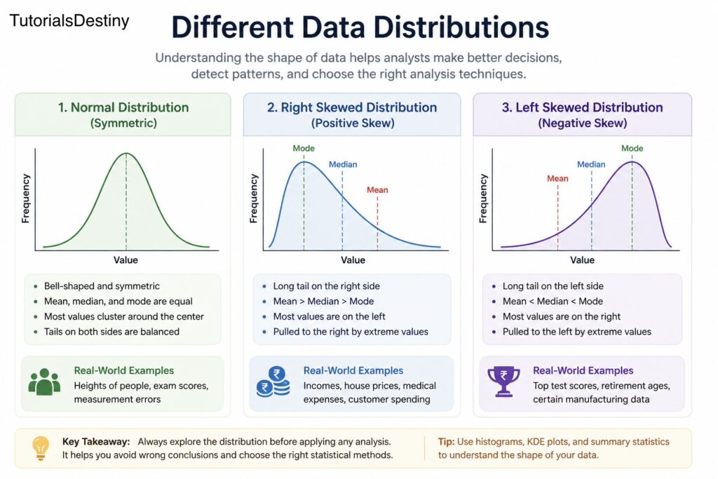
Normal Distribution

The normal distribution is one of the most important and widely studied distributions in statistics.

It is often called the bell-shaped curve because of its symmetrical appearance.

In a normal distribution:

• Most values cluster around the center
• The left and right sides are balanced
• Mean, median, and mode are approximately equal

Characteristics of Normal Distribution

A normal distribution has several important properties:

• Symmetrical shape
• Single central peak
• Gradual decrease on both sides
• Predictable spread around the mean

Many natural and real-world phenomena approximate a normal distribution, including:

• Human height
• Measurement errors
• IQ scores
• Certain biological measurements

Real-World Importance of Normal Distribution

The normal distribution is important because many statistical methods assume data follows this pattern.

For example:

• Confidence intervals
• Hypothesis testing
• Regression analysis

When data is normally distributed, interpretation becomes easier and more predictable.

Skewed Distributions

Not all datasets are balanced. In many real-world situations, values tend to cluster on one side while stretching toward the other.

This creates skewness.

Skewness refers to the asymmetry of a distribution.

There are two main types:

• Right skew (positive skew)
• Left skew (negative skew)

Right-Skewed Distribution

A right-skewed distribution has a long tail extending toward higher values.

\[\text{Mean} > \text{Median} > \text{Mode}\]

In this distribution:

• Most values are concentrated on the left
• A small number of high values pull the distribution to the right

Examples of Right-Skewed Data

Right skew appears frequently in business and economics.

Examples include:

• Income distribution
• House prices
• Online followers
• Customer spending

In these cases, a few extremely high values create a long right tail.

Why Right Skew Matters

When data is right-skewed:

• The mean becomes larger than the median
• Averages may appear misleading
• Outliers strongly influence analysis

This is why understanding the shape of the data is essential before interpreting summary statistics.

Left-Skewed Distribution

A left-skewed distribution has a long tail extending toward lower values.

\[\text{Mean} < \text{Median} < \text{Mode}\]

In this distribution:

• Most values are concentrated on the right
• A few unusually low values pull the distribution leftward

Examples of Left-Skewed Data

Left-skewed distributions are less common but still important.

Examples include:

• Retirement ages in certain professions
• Scores on very easy exams
• Manufacturing quality metrics with occasional low failures

Understanding left skew helps identify situations where lower extreme values influence the dataset.

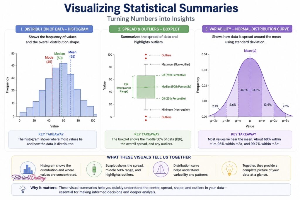
Visualizing Distributions

Visualizations are essential for understanding distribution patterns.

Charts make it easier to identify:

• Symmetry
• Skewness
• Clusters
• Outliers
• Spread

Two of the most common visualization tools are:

• Histograms
• KDE plots

Histograms

A histogram groups numerical values into intervals called bins and displays their frequency.

Histograms help answer questions such as:

• Where are most values concentrated?
• Is the distribution balanced?
• Are there gaps or clusters?

They provide a quick overview of how the dataset behaves.

KDE Plots (Kernel Density Estimation)

KDE plots are smoother versions of histograms.

Instead of showing bars, KDE plots create a continuous curve representing the density of the data.

KDE plots help visualize:

• Peaks in the distribution
• Shape and smoothness
• Density concentration

\[\text{Skewness} = \frac{E[(X-\mu)^3]}{\sigma^3}\]

Interpretation:

• Skewness ≈ 0 → symmetrical distribution
• Positive skewness → right skew
• Negative skewness → left skew

Skewness helps quantify patterns that may already be visible through visualization.

Understanding Kurtosis

Kurtosis measures how sharply peaked or flat a distribution appears.

\[\text{Kurtosis} = \frac{E[(X-\mu)^4]}{\sigma^4}\]

A high kurtosis indicates:

• Sharper peaks
• Heavier tails
• More extreme values

A low kurtosis indicates:

• Flatter distributions
• Fewer extreme values

Kurtosis provides additional insight into the behavior of the dataset.

Real-World Interpretation of Distributions

Understanding distributions is not just a statistical exercise—it has practical importance.

For example:

• In finance, skewed returns may indicate investment risk
• In healthcare, unusual distributions may reveal abnormal conditions
• In e-commerce, customer spending patterns may reveal valuable segments

Distributions help organizations interpret behavior, identify risks, and make better decisions.

Common Mistakes in Distribution Analysis

One common mistake is assuming all data follows a normal distribution. Many real-world datasets are skewed or irregular.

Another mistake is relying only on averages without examining the distribution shape.

Ignoring outliers is also problematic, as extreme values may significantly affect the interpretation of the dataset.

Finally, poor visualization choices can hide important patterns rather than reveal them.

A Practical Example

Imagine an online store analyzing customer purchase amounts.

The average order value may appear high, suggesting strong spending behavior.

However, when the distribution is visualized, the company discovers:

• Most customers place small orders
• A few premium customers place extremely large orders

The distribution is heavily right-skewed.

This insight changes interpretation significantly. Instead of treating all customers equally, the company may focus on retaining premium buyers while also improving engagement among regular customers.

Distribution Analysis in EDA Workflow

Distribution analysis is a core part of Exploratory Data Analysis because it helps reveal the true structure of the data.

It supports:

• Better interpretation of descriptive statistics
• Identification of unusual patterns
• Improved feature engineering
• More accurate modeling decisions

Without understanding distributions, many analytical conclusions become incomplete or misleading.

Preparing for the Next Topic

In the next topic, you will explore relationships between variables through correlation analysis.

You will learn:

• Correlation basics
• Correlation matrices
• Heatmaps
• Difference between correlation and causation
• Confounding variables

This will help you understand how variables interact within a dataset.

Final Thoughts

Distribution analysis provides a deeper understanding of how data behaves. It reveals patterns that averages alone cannot capture and helps identify skewness, variability, and unusual observations.

By learning to interpret distributions correctly, you improve your ability to analyze datasets accurately and make informed decisions.

As you continue through this module, distribution analysis will become one of the most valuable tools in your EDA workflow.

What You Should Take Away

By the end of this topic, you should be able to:

• Understand what data distributions represent
• Differentiate between normal and skewed distributions
• Interpret histograms and KDE plots
• Recognize skewness and kurtosis
• Apply distribution analysis in real-world scenarios

Next Topic

Correlation vs Causation: Understanding Relationships in Data

In the next topic, you will learn how variables interact and why correlation does not always imply causation.

Why Raw Numbers Alone Are Difficult to Understand

Modern datasets often contain thousands or even millions of rows. Looking directly at such large collections of numbers rarely provides meaningful understanding. While the data may contain valuable information, its scale and complexity can make interpretation difficult.

This is where descriptive statistics become essential.

Descriptive statistics help simplify large datasets into understandable summaries. Instead of examining every individual value, these statistical measures allow us to observe patterns, trends, and variability in a compact and meaningful form.

For example, imagine a company analyzing customer purchase amounts from an online store. Looking at thousands of transaction values individually would be overwhelming. However, calculating measures such as the average purchase amount, the most common order size, or the spread of the values immediately provides a clearer picture.

Descriptive statistics act as the first layer of interpretation in data analysis. They help transform raw numerical information into insights that can be explored further.

What are Descriptive Statistics?

Descriptive statistics are methods used to summarize, organize, and describe the main characteristics of a dataset.

These methods do not attempt to predict future outcomes or explain causation. Instead, they focus on describing what currently exists within the data.

Descriptive statistics answer questions such as:

• What is the typical value in the dataset?
• How spread out are the values?
• Which values occur most frequently?
• Are there unusually high or low observations?
• How are values distributed overall?

These summaries provide a foundation for deeper exploration and analysis.

Categories of Descriptive Statistics

Descriptive statistics can generally be divided into two major categories:

Measures of Central Tendency

These measures identify the central or typical value of a dataset.

The three primary measures are:

• Mean
• Median
• Mode

They help describe where the data is centered.

Measures of Variability

These measures describe how spread out the data is.

Important variability measures include:

• Range
• Variance
• Standard deviation
• Percentiles

They help determine whether the data points are closely grouped or widely dispersed.

Together, central tendency and variability provide a balanced understanding of the dataset.

Mean: Understanding the Average

The mean, commonly called the average, is one of the most widely used statistical measures.

It is calculated by adding all values in the dataset and dividing by the number of observations.

\[\text{Mean} = \frac{\sum x}{n}\]

The mean provides a general indication of the center of the dataset.

For example, if five students score 70, 75, 80, 85, and 90 in an exam, the mean score is:

\[\frac{70 + 75 + 80 + 85 + 90}{5} = 80\]

This suggests that the average performance is around 80.

Real-World Importance of Mean

The mean is used extensively in business, finance, healthcare, education, and technology.

Examples include:

• Average customer spending
• Average website traffic
• Average salary
• Average delivery time

Because it considers every value in the dataset, the mean is often useful when the data is relatively balanced.

However, the mean also has limitations.

⚠️ When the Mean Can Be Misleading

One important weakness of the mean is its sensitivity to extreme values, also called outliers.

Consider the following salaries:

|[₹25,000, ₹28,000, ₹30,000, ₹32,000, ₹5,00,000\]

The average salary becomes extremely high because of one unusually large value.

In this case, the mean does not accurately represent what most individuals earn.

This is why descriptive statistics should never rely on a single measure alone.

Median: The Middle Value

The median represents the middle value in an ordered dataset.

To calculate it:

1. Arrange the data in ascending order
2. Identify the middle value

If the dataset has an even number of observations, the median is the average of the two middle values.

\[\text{Median} = \text{Middle Value of Ordered Data}\]

Unlike the mean, the median is not heavily influenced by extreme values.

Why the Median Matters

The median is especially useful for skewed data.

Examples include:

• Income distribution
• House prices
• Social media follower counts

In such datasets, a few extremely large values may distort the average. The median provides a more realistic representation of the typical observation.

For example, if most homes in an area cost between ₹30 lakh and ₹50 lakh, but a few luxury properties cost several crores, the median price gives a better understanding of the housing market than the mean.

Mode: The Most Frequent Value

The mode is the value that appears most frequently in the dataset.

\[\text{Mode} = \text{Most Frequently Occurring Value}\]

Unlike the mean and median, the mode is particularly useful for categorical data.

For example:

• Most purchased product category
• Most common payment method
• Most frequent customer segment

A dataset may have:

• One mode (unimodal)
• Multiple modes (multimodal)
• No mode

Understanding the Difference Between Mean, Median, and Mode

Although these measures all describe central tendency, they provide different perspectives.

• Mean considers all values
• Median focuses on the center position
• Mode identifies frequency

In balanced datasets, these measures are often similar. In skewed datasets, they may differ significantly.

Understanding when to use each measure is an important part of descriptive analysis.

Measuring Variability in Data

Knowing the center of the data is not enough. Two datasets may have the same average but behave very differently.

Consider these examples:

Dataset A:
20, 20, 20, 20, 20

Dataset B:
5, 10, 20, 30, 35

Both datasets may have similar averages, but Dataset B is far more spread out.

This difference is captured through measures of variability.

Range: The Simplest Measure of Spread

The range measures the difference between the highest and lowest values.

\text{Range} = \text{Maximum Value} – \text{Minimum Value}

It provides a quick understanding of how widely values are distributed.

However, the range depends entirely on extreme values and may not always provide a complete picture.

Variance: Measuring Dispersion

Variance measures how far data points are spread from the mean.

A low variance indicates that values are close to the average, while a high variance indicates greater dispersion.

\[\sigma^2 = \frac{\sum (x-\mu)^2}{N}\]

Variance is useful because it quantifies variability mathematically.

However, since variance uses squared values, its units may be difficult to interpret directly.

Standard Deviation: Interpreting Spread More Clearly

Standard deviation is the square root of variance.

\[\sigma = \sqrt{\frac{\sum (x-\mu)^2}{N}}\]

It describes how far, on average, data points lie from the mean.

A small standard deviation suggests that values are clustered closely around the average. A large standard deviation indicates greater variation.

Real-World Examples of Standard Deviation

Standard deviation is widely used in:

• Finance to measure market volatility
• Manufacturing to monitor quality consistency
• Education to analyze score variation
• Healthcare to evaluate measurement stability

Understanding variability helps organizations assess reliability and risk.

Percentiles: Understanding Relative Position

Percentiles divide data into sections based on ranking.

For example:

• The 50th percentile is the median
• The 90th percentile indicates that 90% of values fall below a certain point

Percentiles are useful for:

• Exam rankings
• Income analysis
• Customer segmentation
• Performance benchmarking

They provide context by showing where a value stands relative to the rest of the dataset.

Visualizing Statistical Summaries

Visualization enhances descriptive statistics by making patterns easier to interpret.

Charts such as histograms, boxplots, and distribution curves help reveal:

• Central tendency
• Spread
• Outliers
• Distribution shape

Combining statistical summaries with visualization provides a much deeper understanding than numbers alone.

Common Mistakes in Descriptive Statistics

One common mistake is relying entirely on averages. Averages alone may hide important patterns or distortions.

Another mistake is ignoring variability. Two datasets with the same average may behave very differently depending on how spread out the values are.

Misinterpreting skewed data is another issue. In skewed distributions, the median often provides more meaningful insight than the mean.

Finally, using descriptive statistics without context can lead to misleading conclusions. Numbers should always be interpreted alongside real-world understanding.

A Real-World Case Study

Imagine an e-commerce company analyzing customer spending.

The company calculates the average order value and finds it to be ₹4,500. Initially, this suggests that customers spend heavily.

However, further analysis reveals:

• Most customers spend around ₹1,200–₹1,800
• A small number of premium customers place extremely large orders

The average was inflated by these high-value transactions.

By examining the median and distribution, the company gains a more accurate understanding of customer behavior.

This example demonstrates why multiple descriptive measures must be used together.

Connecting Descriptive Statistics to EDA

Descriptive statistics are one of the first tools used during Exploratory Data Analysis.

They help:

• Summarize large datasets
• Identify patterns quickly
• Detect inconsistencies
• Prepare for deeper analysis

Without descriptive statistics, understanding the overall behavior of a dataset becomes much more difficult.

Preparing for the Next Topic

In the next topic, you will move beyond summary measures and begin exploring how data is distributed.

You will learn:

• Normal vs skewed distributions
• Histograms and KDE plots
• Skewness and kurtosis
• Real-world interpretation of distributions

Understanding distribution analysis will deepen your ability to interpret data patterns accurately.

Final Thoughts

Descriptive statistics provide the foundation for understanding data. They simplify complex datasets into meaningful summaries and reveal important characteristics such as central tendency and variability.

By learning how to interpret measures like mean, median, standard deviation, and percentiles, you develop the ability to explore datasets more confidently and accurately.

These concepts are not just mathematical formulas—they are practical tools used every day in business, science, technology, and research.

As you continue through this module, descriptive statistics will become an essential part of your analytical thinking and data exploration process.

What You Should Take Away

By the end of this topic, you should be able to:

• Understand the purpose of descriptive statistics
• Differentiate between mean, median, and mode
• Interpret measures of variability
• Recognize when averages may be misleading
• Use statistical summaries to explore datasets effectively

Next Topic

Distribution Analysis: Understanding the Shape of Data

In the next topic, you will learn how data distributions influence interpretation, analysis, and decision-making.

Why Understanding Data Comes Before Everything Else

In today’s digital environment, data is generated at an unprecedented scale. Every transaction, click, interaction, and system event produces data that organizations collect and store. This abundance of data creates an opportunity—but also a challenge. The challenge is not in collecting data, but in understanding it.

Many beginners assume that once data is available, the next step is to apply algorithms or build models. However, experienced practitioners know that this approach often leads to unreliable outcomes. Without understanding the structure, quality, and behavior of the data, any analysis built on top of it becomes fragile.

This is why Exploratory Data Analysis (EDA) is not just an optional step—it is a foundational requirement.

EDA is the stage where raw numbers begin to form patterns, and those patterns begin to tell a story. Instead of rushing toward conclusions, it encourages careful observation and structured exploration.

What is Exploratory Data Analysis?

Exploratory Data Analysis is the process of examining a dataset to understand its main characteristics, uncover patterns, detect anomalies, and identify relationships between variables.

It combines statistical thinking with visual interpretation, allowing you to move from raw data to meaningful understanding.

At its core, EDA represents a transformation. Data begins as isolated values but gradually evolves into structured insights that can support decisions. This transition is not automatic—it requires deliberate exploration and interpretation.

EDA helps answer foundational questions:

• What kind of data is present?
• How are values distributed?
• Are there inconsistencies or missing entries?
• Do variables show meaningful relationships?

By answering these questions, the dataset becomes easier to understand and work with.

Types of Exploration in EDA

EDA involves examining data from multiple perspectives to gain a comprehensive view.

• Understanding Individual Variables: Each variable is studied separately to understand its range, distribution, and characteristics.
• Comparing Groups; Data is divided into categories to observe differences between groups.
• Exploring Relationships: Connections between variables are examined to see how they influence each other.
• Identifying Unusual Values: Extreme or unexpected values are analyzed to determine whether they represent errors or important observations.

Each of these perspectives contributes to a deeper understanding of the dataset.

Where EDA Fits in the Data Workflow

EDA plays a central role in the overall data workflow. It acts as a bridge between raw data and deeper analysis.

A typical workflow includes data collection, cleaning, exploration, analysis, and communication. Among these stages, EDA is where the dataset begins to make sense.

Without this step, important details may remain hidden. Patterns may go unnoticed, and errors may persist into later stages. A well-executed EDA ensures that the data is reliable and that the analysis built on it is meaningful.

The Purpose of Exploratory Data Analysis

The goal of EDA is to develop a clear and accurate understanding of the dataset. This involves examining both its structure and its behavior.

EDA helps to:

• Identify different types of variables
• Detect missing or inconsistent values
• Understand how values are distributed
• Recognize patterns and trends
• Explore relationships between variables

These elements combine to create a comprehensive view of the data.

The Role of Questions in EDA

EDA is guided by questions. The depth of understanding you achieve depends on the quality of the questions you ask.

At first, questions may focus on basic structure and summary. Over time, they evolve into more refined inquiries that explore patterns, relationships, and differences.

For example, instead of asking only for averages, it is often more useful to explore how values differ across groups or how they change over time.

This process transforms EDA into an active exploration rather than a passive observation.

From Raw Data to Meaningful Understanding

At the beginning of any data project, a dataset may appear as a collection of unrelated values. Through EDA, these values begin to reveal patterns and structure.

One of the key aspects of this transformation is understanding how data is distributed. Some datasets are balanced and centered, while others are skewed due to real-world factors such as income variation or user behavior.

Recognizing these patterns helps prevent incorrect interpretations and supports better decision-making in later stages.

Exploring Data from Multiple Perspectives

EDA involves examining data from different angles to build a complete understanding.

One approach focuses on individual variables, analyzing their range and distribution. Another involves comparing groups to identify differences between categories. Relationships between variables are also explored to understand how they influence each other.

In addition, unusual values are identified and examined. These may represent errors or important observations, depending on the context.

By combining these perspectives, EDA provides a well-rounded view of the dataset.

The Importance of Visualization

Visualization is a powerful tool in EDA. It allows complex data to be presented in a way that is easy to interpret.

Through charts and graphs, patterns become more visible. Trends, clusters, and outliers can be identified quickly, making it easier to understand the data.

Visualization also improves communication. It allows insights to be shared clearly, even with those who may not be familiar with the underlying data.

Visual tools help to:

• Identify trends and patterns
• Compare values across categories
• Detect outliers or anomalies
• Understand distributions

A Real-World Example: Customer Behavior

To understand how EDA works in practice, consider a dataset containing customer information such as income, spending, and purchase frequency.

Initially, the dataset may appear complex. Through exploration, patterns begin to emerge. You may find that certain groups spend more, or that spending varies across different regions.

You may also discover that some values are unusually high or low, prompting further investigation. These observations gradually build a clearer understanding of customer behavior.

This example highlights how EDA transforms raw data into meaningful insights.

Common Challenges in EDA

While EDA is essential, it requires careful execution.

Missing data can affect accuracy and must be handled appropriately. Patterns must be interpreted cautiously, as not all patterns are meaningful. Data quality issues such as errors or inconsistencies can distort analysis if not addressed.

There is also the risk of bias. It is important to approach data with an open perspective and rely on evidence rather than assumptions.

Being aware of these challenges helps ensure that EDA remains reliable and effective.

EDA as a Foundation for Further Analysis

EDA prepares the dataset for deeper analysis. It ensures that the data is clean, consistent, and well-understood.

Without EDA, analysis may be based on incomplete or misleading information. With EDA, patterns are identified, relationships are understood, and potential issues are resolved.

This makes EDA a critical foundation for any data-driven work.

The Iterative Nature of EDA

EDA is not a one-time activity. As new insights emerge, the process continues.

You may begin with a general overview, then focus on specific variables or patterns. Each step leads to new questions and deeper exploration.

This iterative approach allows for continuous refinement and a more complete understanding of the dataset.

A Guided Thinking Exercise

Imagine you are given a dataset containing product sales data.

Before using any tools, consider how you would explore it:

• What types of products are included?
• How are sales distributed across categories?
• Are there seasonal patterns?
• Which products perform consistently well?

This exercise highlights the importance of structured thinking in EDA. Defining the right questions is the first step toward meaningful analysis.

Preparing for What Comes Next

This topic lays the foundation for the rest of the module. In upcoming sections, you will explore techniques such as descriptive statistics, distribution analysis, and relationship analysis.

These techniques will build on the concepts introduced here and provide practical tools for exploring data effectively.

Final Thoughts

Exploratory Data Analysis is the starting point of meaningful data work. It transforms raw datasets into understandable information and provides clarity for further analysis.

By carefully examining data, identifying patterns, and exploring relationships, EDA enables deeper insights and more informed decisions.

What You Should Take Away

By the end of this topic, you should be able to:

• Understand the role of EDA in the data workflow
• Recognize the importance of exploring data before analysis
• Identify key aspects of a dataset
• Approach data systematically through exploration
• Build a strong foundation for further analysis

Next

Descriptive Statistics: Understanding Data Through Summary Measures

In the next topic, you will learn how to summarize and interpret data using statistical measures such as mean, median, mode, variance, standard deviation, and percentiles. You will also understand when averages can be misleading and how descriptive statistics help uncover the true nature of a dataset.

---

Module 3: Data Cleaning & Wrangling — Page 5

---

Introduction: Turning Clean Data into Meaningful Insights

By this point in your journey, you’ve already handled missing values and learned how to filter, group, and merge datasets. Your data is cleaner and more structured—but it’s still not fully ready to generate deep insights or power strong models.

This is where feature creation and data transformation come into play.

In real-world data analysis, raw data rarely contains all the signals you need. Instead, analysts create new variables—called features—that better represent patterns, relationships, and behaviors hidden within the data. Alongside this, transformations help ensure that your data is in the right format and scale for meaningful analysis.

This step is often what separates a basic analysis from a powerful one. Many experienced data professionals will tell you that the quality of your features matters more than the complexity of your model. In other words, better inputs lead to better outputs.

---

Understanding Feature Engineering

Feature engineering is essentially about thinking beyond the dataset as it is given. Instead of passively analyzing columns, you actively reshape them to reflect meaningful concepts.

For example, a dataset might include:

• Transaction dates
• Revenue values
• Product categories

Individually, these are useful—but limited. When you start deriving features such as monthly revenue, profit margins, or customer segments, the dataset becomes far more expressive.

At a conceptual level, feature engineering helps you:

• Align data with business questions
• Reveal hidden relationships
• Improve both analysis and model performance

This is why, in many real-world projects, feature engineering consumes a significant portion of the analyst’s time.

---

Creating New Features from Existing Data

One of the most intuitive ways to create features is through simple mathematical transformations. Even basic arithmetic operations can significantly enhance how data is interpreted.

For instance, calculating profit from revenue and cost immediately introduces a more meaningful metric:

df['profit'] = df['revenue'] - df['cost']

Taking it a step further, ratio-based features such as profit margin provide normalized insights:

df['profit_margin'] = df['profit'] / df['revenue']

These derived features are often more useful than raw numbers because they allow comparisons across different scales.

Beyond simple calculations, you can also create features using grouped context. This means incorporating information about the broader group a data point belongs to.

df['region_avg_sales'] = df.groupby('region')['sales'].transform('mean')

This approach helps answer questions like:

• Is this sale above or below the regional average?
• How does this customer compare to others in the same segment?

These kinds of contextual features are extremely valuable in both analysis and modeling.

---

Working with Date and Time Data

Date columns are often underutilized, especially by beginners. However, they contain a wealth of information that can significantly improve your analysis.

Once converted into a proper datetime format, you can extract multiple components:

df['date'] = pd.to_datetime(df['date'])
df['year'] = df['date'].dt.year
df['month'] = df['date'].dt.month
df['weekday'] = df['date'].dt.day_name()

Instead of treating time as a single variable, you now have multiple dimensions to analyze.

This allows you to explore patterns such as:

• Monthly or seasonal trends
• Weekday vs weekend behavior
• Year-over-year growth

In business scenarios, these insights are critical. For example, identifying seasonal demand patterns can directly influence inventory and marketing strategies.

---

Transforming Categorical Variables

Categorical data appears in almost every dataset, whether it’s product categories, regions, or customer segments. While these variables are easy to understand conceptually, they often need to be transformed for analysis and modeling.

A common technique is one-hot encoding, which converts each category into a binary column:

pd.get_dummies(df['category'])

This approach works well when categories have no inherent order.

In contrast, label encoding assigns numeric values to categories. This is more suitable when there is a natural ranking or order.

When working with categorical data, it’s important to remember:

• The encoding method should match the nature of the data
• Incorrect encoding can distort relationships
• Simpler representations are often more interpretable

---

Binning and Discretization

Sometimes, continuous variables are easier to understand when grouped into categories. This process is known as binning.

For example:

df['age_group'] = pd.cut(df['age'], bins=5)

Instead of analyzing exact age values, you now work with ranges. This simplifies interpretation and makes patterns more visible.

Binning is particularly useful when:

• You want to segment users or products
• Exact values are less important than ranges
• You are preparing data for business reporting

However, it’s important not to overuse binning, as it can reduce detail if applied unnecessarily.

---

Scaling and Normalization

In many datasets, different features operate on completely different scales. For example, revenue might be in thousands, while quantity sold might be in single digits.

Such differences can create imbalance, especially in machine learning models.

Two common techniques are:

• Normalization, which rescales values between 0 and 1
• Standardization, which centers data around the mean

(df - df.min()) / (df.max() - df.min())
(df - df.mean()) / df.std()

These transformations ensure that no single feature dominates others purely due to scale.

In general, scaling becomes important when:

• Working with distance-based models
• Comparing variables with different units
• Preparing data for advanced modeling

---

Handling Skewed Data

Real-world data is rarely perfectly distributed. Many variables, especially financial ones like revenue or income, tend to be heavily skewed.

This means that a small number of values dominate the dataset, which can distort analysis.

A common way to address this is through log transformation:

df['log_revenue'] = np.log(df['revenue'])

This transformation compresses large values and spreads out smaller ones, making patterns easier to observe.

You should consider transformation when:

• Data has extreme outliers
• Distribution is highly skewed
• Visualization appears uneven

---

Creating Interaction Features

Sometimes, the relationship between variables is more important than the variables themselves.

For example:

df['sales_per_customer'] = df['sales'] / df['customers']

This new feature captures efficiency rather than absolute values.

Interaction features are useful because they:

• Combine multiple dimensions into one
• Reveal deeper insights
• Often improve predictive performance

---

Feature Selection: Keeping What Matters

While creating features is important, using too many can be counterproductive. Not every feature adds value, and some may introduce noise.

It’s often necessary to remove:

• Redundant columns
• Highly correlated features
• Irrelevant identifiers (like IDs)

Feature selection helps:

• Simplify analysis
• Improve model performance
• Reduce computational complexity

A good analyst focuses not just on creating features—but on keeping the right ones.

---

A Practical Workflow

To bring everything together, let’s look at how feature engineering fits into a real workflow.

Imagine you are working with a sales dataset. A structured approach might look like this:

• Convert date columns into datetime format
• Extract time-based features such as month and weekday
• Create business metrics like profit and margin
• Encode categorical variables for analysis
• Normalize numerical features where needed
• Add group-level context using aggregations

This step-by-step process transforms raw data into something that is far more informative and actionable.

---

Common Mistakes to Avoid

Feature engineering is powerful, but it’s also easy to misuse. Some common pitfalls include:

• Creating too many features without clear purpose
• Ignoring business context while designing features
• Applying transformations blindly
• Introducing data leakage in modeling scenarios

The key is to stay intentional. Every transformation should answer the question: “Does this make my data more meaningful?”

---

Key Takeaways

Feature creation and transformation are central to effective data analysis. They allow you to reshape raw data into forms that better reflect real-world patterns and relationships.

At this stage, you should be comfortable:

• Creating new features from existing columns
• Extracting useful information from dates
• Transforming categorical and numerical data
• Applying scaling and handling skewed distributions
• Thinking critically about which features actually matter

---

Final Insight

Good analysis doesn’t come from more data—it comes from better representation of data.

Feature engineering is where raw information becomes insight-ready.

---

What’s Next?

In the next module, you will move into:

Exploratory Data Analysis (EDA)

This is where you begin visualizing and interpreting your transformed data to uncover trends, patterns, and actionable insights.

---

---

---

Introduction: From Clean Data to Useful Insights

By now, your data is cleaner. You’ve handled missing values and ensured that your dataset is more consistent and reliable. But clean data alone does not automatically produce insights.

To answer real questions, you need to actively work with your data—selecting relevant portions, summarizing patterns, and combining multiple sources. This is where filtering, grouping, and merging become essential.

These operations form the backbone of practical data analysis. Whether you are building dashboards, analyzing customer behavior, or preparing data for models, you will constantly rely on these techniques to reshape your dataset into something meaningful.

This page marks an important transition: you move from cleaning data to using data.

---

Understanding Data Manipulation

Data manipulation is the process of transforming a dataset so that it can answer specific questions. Instead of working with the entire dataset at once, you break it down into smaller, more relevant pieces.

In practice, this usually involves:

• Selecting specific rows or columns
• Aggregating data to identify patterns
• Combining multiple datasets into one

These steps may seem simple individually, but together they form the core workflow of almost every data analysis project.

---

Filtering Data: Focusing on What Matters

Filtering allows you to extract only the data that is relevant to your analysis. In real-world scenarios, you rarely work with the entire dataset—you focus on subsets that help answer a specific question.

For example, if you are analyzing sales performance, you might only want to look at transactions above a certain value or within a specific region.

In pandas, filtering is typically done using conditions:

df[df['sales'] > 1000]

This returns only the rows where sales exceed 1000.

You can also combine multiple conditions to refine your selection:

df[(df['sales'] > 1000) & (df['region'] == 'West')]

This kind of filtering is powerful because it allows you to isolate very specific segments of your data.

---

Making Filtering More Readable

As conditions become more complex, readability becomes important. One alternative is using the query() method:

df.query("sales > 1000 and region == 'West'")

This approach often feels more intuitive, especially when working with multiple conditions.

---

Common Filtering Scenarios

Filtering is used in many everyday analysis tasks. For example:

• Identifying high-value customers
• Selecting data for a specific time period
• Removing outliers or invalid records
• Analyzing performance within a category

The key idea is simple: filtering helps you focus your analysis on what actually matters.

---

Selecting and Organizing Columns

In addition to filtering rows, you often need to work with only a subset of columns. Large datasets can contain many variables, not all of which are relevant to your current task.

Selecting specific columns makes your analysis cleaner and easier to understand:

df[['sales', 'profit']]

At times, you may also want to remove unnecessary columns:

df.drop(columns=['unnecessary_column'])

Reducing the dataset to only what you need improves both performance and clarity.

---

Sorting Data for Better Understanding

Sorting is a simple yet powerful way to explore your data. By ordering values, you can quickly identify trends, extremes, and anomalies.

For example:

df.sort_values(by='sales', ascending=False)

This helps you identify top-performing records.

Sorting by multiple columns can provide even deeper insights:

df.sort_values(by=['region', 'sales'])

This allows you to compare performance within each group.

---

Grouping Data: Discovering Patterns

While filtering helps you narrow down data, grouping helps you summarize it.

Grouping allows you to split data into categories and apply calculations to each group. This is one of the most important concepts in data analysis because it transforms raw data into meaningful summaries.

For example, calculating total sales per region:

df.groupby('region')['sales'].sum()

This gives you a clear view of how different regions are performing.

---

Aggregating Data

Grouping becomes even more powerful when combined with aggregation functions. Common operations include:

• Summing values to get totals
• Calculating averages to understand typical behavior
• Counting entries to measure frequency

You can also apply multiple aggregations at once:

df.groupby('region').agg({
    'sales': 'sum',
    'profit': 'mean'
})

This provides a richer summary of your data.

---

Grouping by Multiple Dimensions

Real-world data often involves multiple variables. You can group by more than one column to get deeper insights:

df.groupby(['region', 'category'])['sales'].sum()

This allows you to analyze how categories perform within each region.

---

Keeping Results Structured

After grouping, the result may have a hierarchical index. Resetting the index makes the output easier to work with:

df.groupby('region')['sales'].sum().reset_index()

---

Why Grouping Matters

Grouping is where data starts to answer questions like:

• Which region generates the most revenue?
• Which product category performs best?
• What is the average customer spending?

This is a major step toward real insight generation.

---

Transforming Data Within Groups

Sometimes, you don’t want to reduce data—you want to enrich it with group-level information.

This is where transform() becomes useful:

df['region_avg'] = df.groupby('region')['sales'].transform('mean')

Now, each row includes the average sales for its region.

This allows you to compare individual performance against group benchmarks, which is extremely valuable in analysis.

---

Merging Data: Combining Multiple Sources

In real-world projects, data rarely exists in a single table. Instead, it is spread across multiple datasets—customers, orders, products, and more.

Merging allows you to combine these datasets into one.

---

Understanding Joins

The most common way to merge data in pandas is using merge().

An inner join keeps only matching records:

pd.merge(df1, df2, on='key', how='inner')

A left join keeps all records from the first dataset:

pd.merge(df1, df2, on='key', how='left')

Each type of join serves a different purpose, depending on your analysis.

---

Choosing the Right Join

Selecting the correct join is critical. The wrong choice can:

• Remove important data
• Introduce missing values
• Duplicate records

This is why merging should always be done carefully and verified afterward.

---

Handling Missing Data After Merge

After merging, you may notice new missing values. This happens when records don’t match across datasets.

For example:

• A customer without any orders
• A product that hasn’t been sold

This connects directly to what you learned in the previous page about handling missing values.

---

Concatenation: Another Way to Combine Data

Not all data combinations require merging. Sometimes, you simply need to stack datasets together.

This is done using concatenation:

pd.concat([df1, df2])

Concatenation is useful when:

• Combining similar datasets
• Appending new data
• Working with multiple files

Unlike merging, it does not rely on keys.

---

A Practical Workflow

To understand how these operations come together, consider a typical analysis scenario.

You might:

• Filter data for a specific time period
• Select relevant columns
• Merge customer and transaction datasets
• Group data by region or category
• Calculate key metrics such as total sales or average profit
• Sort results to identify top performers

This workflow reflects how analysts approach real-world problems.

---

Common Mistakes to Avoid

Even though these operations are fundamental, mistakes can easily occur.

Some common issues include:

• Using incorrect filtering conditions
• Forgetting parentheses in logical expressions
• Choosing the wrong join type
• Not checking for duplicates after merging
• Ignoring index structure after grouping

Being aware of these pitfalls helps you avoid incorrect conclusions.

---

Key Takeaways

Filtering, grouping, and merging are essential tools for transforming raw data into meaningful insights.

At this stage, you should be comfortable:

• Filtering datasets using conditions
• Selecting and organizing relevant data
• Grouping data to uncover patterns
• Applying aggregation functions
• Merging datasets correctly
• Building structured workflows for analysis

---

Final Insight

Cleaning data prepares it for use.
Manipulating data is what unlocks its value.

These techniques are the foundation of real-world data analysis.

---

What’s Next?

In the next page, you will move into:

Feature Creation & Data Transformation

This is where you begin engineering new variables that improve both analysis and model performance.

---

---

Introduction: Why Missing Data Deserves Serious Attention

In almost every real-world dataset, missing values are inevitable. Whether you are analyzing customer transactions, product data, or survey responses, you will encounter gaps—fields left blank, values not recorded, or information that simply doesn’t exist.

At first glance, missing data may seem like a minor inconvenience. However, it can significantly impact the quality of your analysis. If handled poorly, missing values can distort trends, bias results, and lead to incorrect conclusions.

This is why handling missing data is not just a technical step—it is a critical part of analytical thinking.

Instead of asking “How do I remove missing values?”, a better question is:

“What do these missing values represent, and how should I handle them responsibly?”

This shift in thinking is what separates basic data cleaning from professional-level analysis.

---

Understanding Missing Values

Missing values represent the absence of data where a value is expected. In Python, especially when using pandas, missing values are typically represented as:

• NaN (Not a Number)
• None (commonly in object-type columns)

Although these placeholders look simple, they carry deeper meaning. A missing value is not just “empty”—it often reflects something about how the data was collected, processed, or recorded.

For example, a missing value in a customer dataset might mean:

• The user skipped an optional field
• The system failed to record information
• The data was lost during merging

Each of these scenarios requires a different approach. Treating all missing values the same is one of the most common mistakes beginners make.

---

Why Missing Data Matters in Analysis

Before deciding how to handle missing values, it’s important to understand the consequences of ignoring them.

Missing data can affect your analysis in several ways:

• It can distort averages and statistical summaries
• It can create misleading patterns in visualizations
• It can break machine learning models that require complete data
• It can introduce bias if the missingness is not random

For example, if high-income individuals are more likely to skip income-related fields, simply ignoring those missing values could lead you to underestimate average income.

This is why handling missing data requires both technical skill and contextual judgment.

---

Types of Missing Data

To make better decisions, analysts classify missing data based on why it is missing. While you don’t always need to formally label each case, understanding these categories improves your intuition.

---

Missing Completely at Random (MCAR)

This occurs when the missing values have no relationship with any variable in the dataset.

For instance, a few records might be missing due to a random system glitch. In such cases, the missing data does not introduce bias.

In practice, this is the easiest type to handle because you can often remove those rows without affecting your analysis significantly.

---

Missing at Random (MAR)

Here, the missingness is related to another variable in the dataset.

For example, younger users may be less likely to fill in income details. In this case, the missing values are not random—they are influenced by another feature.

Handling this type of missing data requires more care because patterns exist behind the missing values.

---

Missing Not at Random (MNAR)

This is the most complex situation. The missingness depends on the value itself.

For example:

• People with higher income choose not to disclose it
• Dissatisfied customers skip feedback questions

In such cases, the absence of data carries meaning. Ignoring it can lead to serious bias.

---

Detecting Missing Values in pandas

Before you can handle missing data, you need to identify where it exists and how extensive it is.

In pandas, this process is straightforward but extremely important.

---

Identifying Missing Values

You can detect missing values using:

df.isnull()

This returns a DataFrame showing True where values are missing.

---

Counting Missing Values

To get a clearer overview, you can count missing values per column:

df.isnull().sum()

This helps you quickly identify which columns need attention.

---

Measuring Missing Data Percentage

Counts alone can be misleading, especially in large datasets. Calculating percentages provides better context:

df.isnull().mean() * 100

This tells you how significant the missing data problem is.

---

Interpreting Missing Data

Once you detect missing values, the next step is interpretation.

Instead of jumping to action, take a moment to analyze:

• Is the missing data concentrated in specific columns?
• Do certain rows have multiple missing values?
• Is there a pattern linked to categories or time?

This step is often overlooked, but it is critical. Good analysts spend time understanding the problem before applying solutions.

---

Strategy 1: Dropping Missing Data

One of the simplest ways to handle missing values is to remove them entirely.

---

Dropping Rows

df.dropna()

This removes any row containing missing values.

---

Dropping Columns

df.dropna(axis=1)

This removes columns with missing data.

---

When Dropping Makes Sense

Dropping data is appropriate when:

• The amount of missing data is very small
• The dataset is large enough to absorb the loss
• The missing values appear random

---

Limitations of Dropping

While simple, this approach has drawbacks. Removing too much data can reduce the quality of your analysis and may introduce bias if the missingness is not random.

Because of this, dropping should be used carefully—not as a default solution.

---

Strategy 2: Filling Missing Values (Imputation)

Instead of removing data, you can replace missing values with estimated ones. This process is called imputation.

---

Mean and Median Imputation

For numerical data, a common approach is to use the mean or median:

df['column'] = df['column'].fillna(df['column'].mean())

or

df['column'] = df['column'].fillna(df['column'].median())

The median is often preferred when the data is skewed.

---

Mode Imputation

For categorical data, the most frequent value can be used:

df['column'] = df['column'].fillna(df['column'].mode()[0])

---

Understanding the Trade-Off

Imputation allows you to retain data, but it introduces assumptions. You are essentially estimating missing values, which may not always reflect reality.

Because of this, imputation should be used thoughtfully, especially in sensitive analyses.

---

Strategy 3: Forward Fill and Backward Fill

In time-based data, missing values often occur in sequences. In such cases, you can propagate nearby values.

---

Forward Fill

df.fillna(method='ffill')

This fills missing values using the last known value.

---

Backward Fill

df.fillna(method='bfill')

This uses the next available value.

---

When This Works Well

These methods are particularly useful for:

• Time-series data
• Sensor readings
• Sequential logs

However, they should not be applied to unrelated data, as they assume continuity.

---

Strategy 4: Conditional Imputation

More advanced handling involves filling missing values based on specific conditions or groups.

For example, instead of filling missing salary values with a global average, you might fill them based on job role or region.

This approach respects the structure of the data and often produces more realistic results.

---

Strategy 5: Keeping Missing Values as Information

In some cases, missing values themselves carry meaning and should not be removed or replaced.

Instead, you can create a new feature to indicate missingness:

df['is_missing'] = df['column'].isnull()

This allows you to capture patterns where missing data is informative.

For example, users who skip certain fields may behave differently from those who fill them.

---

Choosing the Right Approach

There is no universal rule for handling missing values. The right approach depends on context.

A practical way to think about it is:

• Small, random missing data → consider dropping
• Moderate missing data → consider imputation
• Patterned missing data → investigate further
• Meaningful missing data → preserve as a feature

The key is to combine technical methods with logical reasoning.

---

Common Mistakes to Avoid

Handling missing values is deceptively simple, which is why mistakes are common.

Some pitfalls to watch out for include:

• Dropping large portions of data without analysis
• Blindly filling values without understanding distribution
• Ignoring patterns in missing data
• Treating all columns the same
• Not validating results after cleaning

Avoiding these mistakes will significantly improve the quality of your work.

---

A Practical Workflow

A structured approach helps ensure consistency when handling missing data.

A typical workflow looks like this:

• Detect missing values
• Measure their extent
• Analyze patterns and context
• Choose an appropriate strategy
• Apply the solution
• Validate the dataset

This process reflects how real analysts approach data cleaning—not as a quick fix, but as a thoughtful, iterative step.

---

Key Takeaways

Handling missing values is one of the most important skills in data analysis.

At this stage, you should understand:

• Missing data is unavoidable in real-world datasets
• The reason behind missingness matters more than the absence itself
• Different strategies exist, each with trade-offs
• Good handling requires judgment, not just code

---

Final Insight

Missing data is not just a problem to fix—it is information to interpret.

The goal is not to make your dataset “perfect,” but to make it reliable enough for meaningful analysis.

---

What’s Next?

You’ve learned how to handle missing values effectively, but there’s another foundational issue that can silently break your analysis—incorrect data types.

Even clean-looking data can behave incorrectly if values are stored in the wrong format.

👉 Next: Data Types & Conversions
Learn how to identify, fix, and convert data types to ensure your dataset behaves correctly during analysis.

---