Why Raw Numbers Alone Are Difficult to Understand

Modern datasets often contain thousands or even millions of rows. Looking directly at such large collections of numbers rarely provides meaningful understanding. While the data may contain valuable information, its scale and complexity can make interpretation difficult.

This is where descriptive statistics become essential.

Descriptive statistics help simplify large datasets into understandable summaries. Instead of examining every individual value, these statistical measures allow us to observe patterns, trends, and variability in a compact and meaningful form.

For example, imagine a company analyzing customer purchase amounts from an online store. Looking at thousands of transaction values individually would be overwhelming. However, calculating measures such as the average purchase amount, the most common order size, or the spread of the values immediately provides a clearer picture.

Descriptive statistics act as the first layer of interpretation in data analysis. They help transform raw numerical information into insights that can be explored further.

What are Descriptive Statistics?

Descriptive statistics are methods used to summarize, organize, and describe the main characteristics of a dataset.

These methods do not attempt to predict future outcomes or explain causation. Instead, they focus on describing what currently exists within the data.

Descriptive statistics answer questions such as:

• What is the typical value in the dataset?
• How spread out are the values?
• Which values occur most frequently?
• Are there unusually high or low observations?
• How are values distributed overall?

These summaries provide a foundation for deeper exploration and analysis.

Categories of Descriptive Statistics

Descriptive statistics can generally be divided into two major categories:

Measures of Central Tendency

These measures identify the central or typical value of a dataset.

The three primary measures are:

• Mean
• Median
• Mode

They help describe where the data is centered.

Measures of Variability

These measures describe how spread out the data is.

Important variability measures include:

• Range
• Variance
• Standard deviation
• Percentiles

They help determine whether the data points are closely grouped or widely dispersed.

Together, central tendency and variability provide a balanced understanding of the dataset.

Mean: Understanding the Average

The mean, commonly called the average, is one of the most widely used statistical measures.

It is calculated by adding all values in the dataset and dividing by the number of observations.

\[\text{Mean} = \frac{\sum x}{n}\]

The mean provides a general indication of the center of the dataset.

For example, if five students score 70, 75, 80, 85, and 90 in an exam, the mean score is:

\[\frac{70 + 75 + 80 + 85 + 90}{5} = 80\]

This suggests that the average performance is around 80.

Real-World Importance of Mean

The mean is used extensively in business, finance, healthcare, education, and technology.

Examples include:

• Average customer spending
• Average website traffic
• Average salary
• Average delivery time

Because it considers every value in the dataset, the mean is often useful when the data is relatively balanced.

However, the mean also has limitations.

⚠️ When the Mean Can Be Misleading

One important weakness of the mean is its sensitivity to extreme values, also called outliers.

Consider the following salaries:

|[₹25,000, ₹28,000, ₹30,000, ₹32,000, ₹5,00,000\]

The average salary becomes extremely high because of one unusually large value.

In this case, the mean does not accurately represent what most individuals earn.

This is why descriptive statistics should never rely on a single measure alone.

Median: The Middle Value

The median represents the middle value in an ordered dataset.

To calculate it:

1. Arrange the data in ascending order
2. Identify the middle value

If the dataset has an even number of observations, the median is the average of the two middle values.

\[\text{Median} = \text{Middle Value of Ordered Data}\]

Unlike the mean, the median is not heavily influenced by extreme values.

Why the Median Matters

The median is especially useful for skewed data.

Examples include:

• Income distribution
• House prices
• Social media follower counts

In such datasets, a few extremely large values may distort the average. The median provides a more realistic representation of the typical observation.

For example, if most homes in an area cost between ₹30 lakh and ₹50 lakh, but a few luxury properties cost several crores, the median price gives a better understanding of the housing market than the mean.

Mode: The Most Frequent Value

The mode is the value that appears most frequently in the dataset.

\[\text{Mode} = \text{Most Frequently Occurring Value}\]

Unlike the mean and median, the mode is particularly useful for categorical data.

For example:

• Most purchased product category
• Most common payment method
• Most frequent customer segment

A dataset may have:

• One mode (unimodal)
• Multiple modes (multimodal)
• No mode

Understanding the Difference Between Mean, Median, and Mode

Although these measures all describe central tendency, they provide different perspectives.

• Mean considers all values
• Median focuses on the center position
• Mode identifies frequency

In balanced datasets, these measures are often similar. In skewed datasets, they may differ significantly.

Understanding when to use each measure is an important part of descriptive analysis.

Measuring Variability in Data

Knowing the center of the data is not enough. Two datasets may have the same average but behave very differently.

Consider these examples:

Dataset A:
20, 20, 20, 20, 20

Dataset B:
5, 10, 20, 30, 35

Both datasets may have similar averages, but Dataset B is far more spread out.

This difference is captured through measures of variability.

Range: The Simplest Measure of Spread

The range measures the difference between the highest and lowest values.

\text{Range} = \text{Maximum Value} – \text{Minimum Value}

It provides a quick understanding of how widely values are distributed.

However, the range depends entirely on extreme values and may not always provide a complete picture.

Variance: Measuring Dispersion

Variance measures how far data points are spread from the mean.

A low variance indicates that values are close to the average, while a high variance indicates greater dispersion.

\[\sigma^2 = \frac{\sum (x-\mu)^2}{N}\]

Variance is useful because it quantifies variability mathematically.

However, since variance uses squared values, its units may be difficult to interpret directly.

Standard Deviation: Interpreting Spread More Clearly

Standard deviation is the square root of variance.

\[\sigma = \sqrt{\frac{\sum (x-\mu)^2}{N}}\]

It describes how far, on average, data points lie from the mean.

A small standard deviation suggests that values are clustered closely around the average. A large standard deviation indicates greater variation.

Real-World Examples of Standard Deviation

Standard deviation is widely used in:

• Finance to measure market volatility
• Manufacturing to monitor quality consistency
• Education to analyze score variation
• Healthcare to evaluate measurement stability

Understanding variability helps organizations assess reliability and risk.

Percentiles: Understanding Relative Position

Percentiles divide data into sections based on ranking.

For example:

• The 50th percentile is the median
• The 90th percentile indicates that 90% of values fall below a certain point

Percentiles are useful for:

• Exam rankings
• Income analysis
• Customer segmentation
• Performance benchmarking

They provide context by showing where a value stands relative to the rest of the dataset.

Visualizing Statistical Summaries

Visualization enhances descriptive statistics by making patterns easier to interpret.

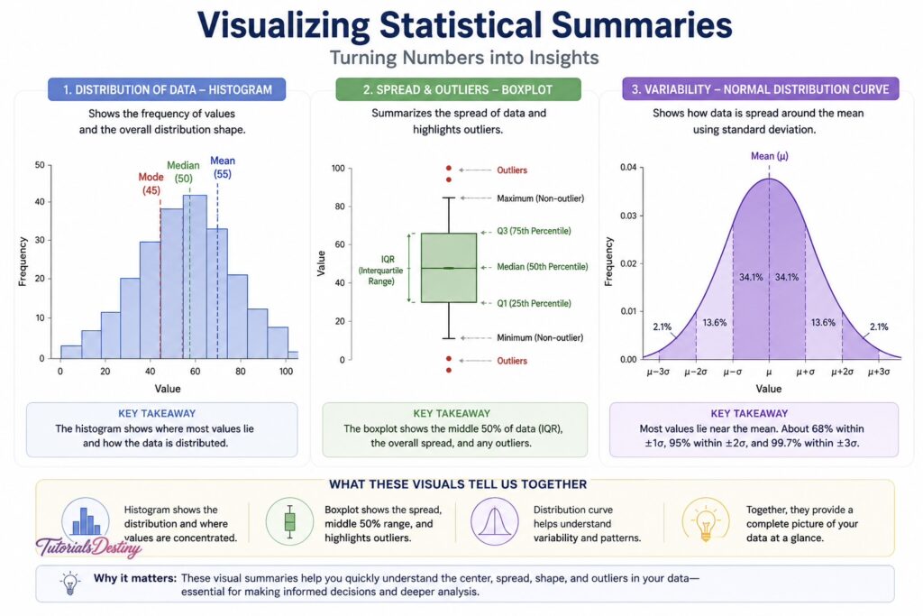
Charts such as histograms, boxplots, and distribution curves help reveal:

• Central tendency
• Spread
• Outliers
• Distribution shape

Combining statistical summaries with visualization provides a much deeper understanding than numbers alone.

Common Mistakes in Descriptive Statistics

One common mistake is relying entirely on averages. Averages alone may hide important patterns or distortions.

Another mistake is ignoring variability. Two datasets with the same average may behave very differently depending on how spread out the values are.

Misinterpreting skewed data is another issue. In skewed distributions, the median often provides more meaningful insight than the mean.

Finally, using descriptive statistics without context can lead to misleading conclusions. Numbers should always be interpreted alongside real-world understanding.

A Real-World Case Study

Imagine an e-commerce company analyzing customer spending.

The company calculates the average order value and finds it to be ₹4,500. Initially, this suggests that customers spend heavily.

However, further analysis reveals:

• Most customers spend around ₹1,200–₹1,800
• A small number of premium customers place extremely large orders

The average was inflated by these high-value transactions.

By examining the median and distribution, the company gains a more accurate understanding of customer behavior.

This example demonstrates why multiple descriptive measures must be used together.

Connecting Descriptive Statistics to EDA

Descriptive statistics are one of the first tools used during Exploratory Data Analysis.

They help:

• Summarize large datasets
• Identify patterns quickly
• Detect inconsistencies
• Prepare for deeper analysis

Without descriptive statistics, understanding the overall behavior of a dataset becomes much more difficult.

Preparing for the Next Topic

In the next topic, you will move beyond summary measures and begin exploring how data is distributed.

You will learn:

• Normal vs skewed distributions
• Histograms and KDE plots
• Skewness and kurtosis
• Real-world interpretation of distributions

Understanding distribution analysis will deepen your ability to interpret data patterns accurately.

Final Thoughts

Descriptive statistics provide the foundation for understanding data. They simplify complex datasets into meaningful summaries and reveal important characteristics such as central tendency and variability.

By learning how to interpret measures like mean, median, standard deviation, and percentiles, you develop the ability to explore datasets more confidently and accurately.

These concepts are not just mathematical formulas—they are practical tools used every day in business, science, technology, and research.

As you continue through this module, descriptive statistics will become an essential part of your analytical thinking and data exploration process.

What You Should Take Away

By the end of this topic, you should be able to:

• Understand the purpose of descriptive statistics
• Differentiate between mean, median, and mode
• Interpret measures of variability
• Recognize when averages may be misleading
• Use statistical summaries to explore datasets effectively

Next Topic

Distribution Analysis: Understanding the Shape of Data

In the next topic, you will learn how data distributions influence interpretation, analysis, and decision-making.